Code
library(tidyverse)
library(readxl)
library(ggplot2)
library(stats)


knitr::opts_chunk$set(echo = TRUE)Niyati Sharma
October 3, 2022
# A tibble: 725 × 6
LungCap Age Height Smoke Gender Caesarean
<dbl> <dbl> <dbl> <chr> <chr> <chr>
1 6.48 6 62.1 no male no
2 10.1 18 74.7 yes female no
3 9.55 16 69.7 no female yes
4 11.1 14 71 no male no
5 4.8 5 56.9 no male no
6 6.22 11 58.7 no female no
7 4.95 8 63.3 no male yes
8 7.32 11 70.4 no male no
9 8.88 15 70.5 no male no
10 6.8 11 59.2 no male no
# … with 715 more rows##A
The histogram looks close to normal distributed.
The probability density of the female is higher than the males.
# A tibble: 2 × 2
Smoke mean
<chr> <dbl>
1 no 7.77
2 yes 8.65
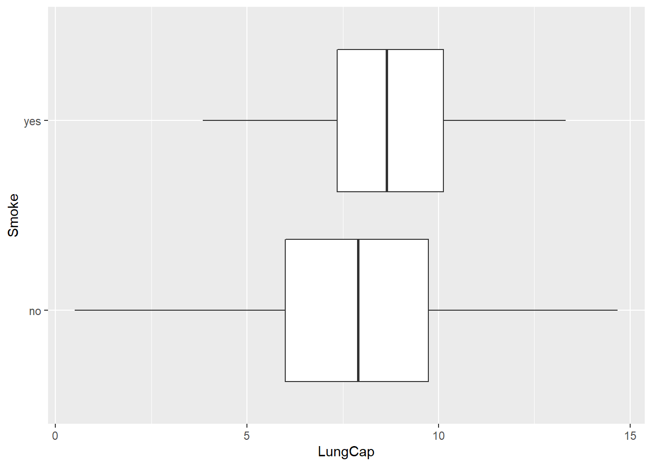
From this sample, it appears that smokers have a higher mean lung capacity than non-smokers.
# A tibble: 725 × 7
LungCap Age Height Smoke Gender Caesarean Category
<dbl> <dbl> <dbl> <chr> <chr> <chr> <fct>
1 6.48 6 62.1 no male no 13 and under
2 10.1 18 74.7 yes female no 18 or over
3 9.55 16 69.7 no female yes 16-17
4 11.1 14 71 no male no 14-15
5 4.8 5 56.9 no male no 13 and under
6 6.22 11 58.7 no female no 13 and under
7 4.95 8 63.3 no male yes 13 and under
8 7.32 11 70.4 no male no 13 and under
9 8.88 15 70.5 no male no 14-15
10 6.8 11 59.2 no male no 13 and under
# … with 715 more rows`stat_bin()` using `bins = 30`. Pick better value with `binwidth`.
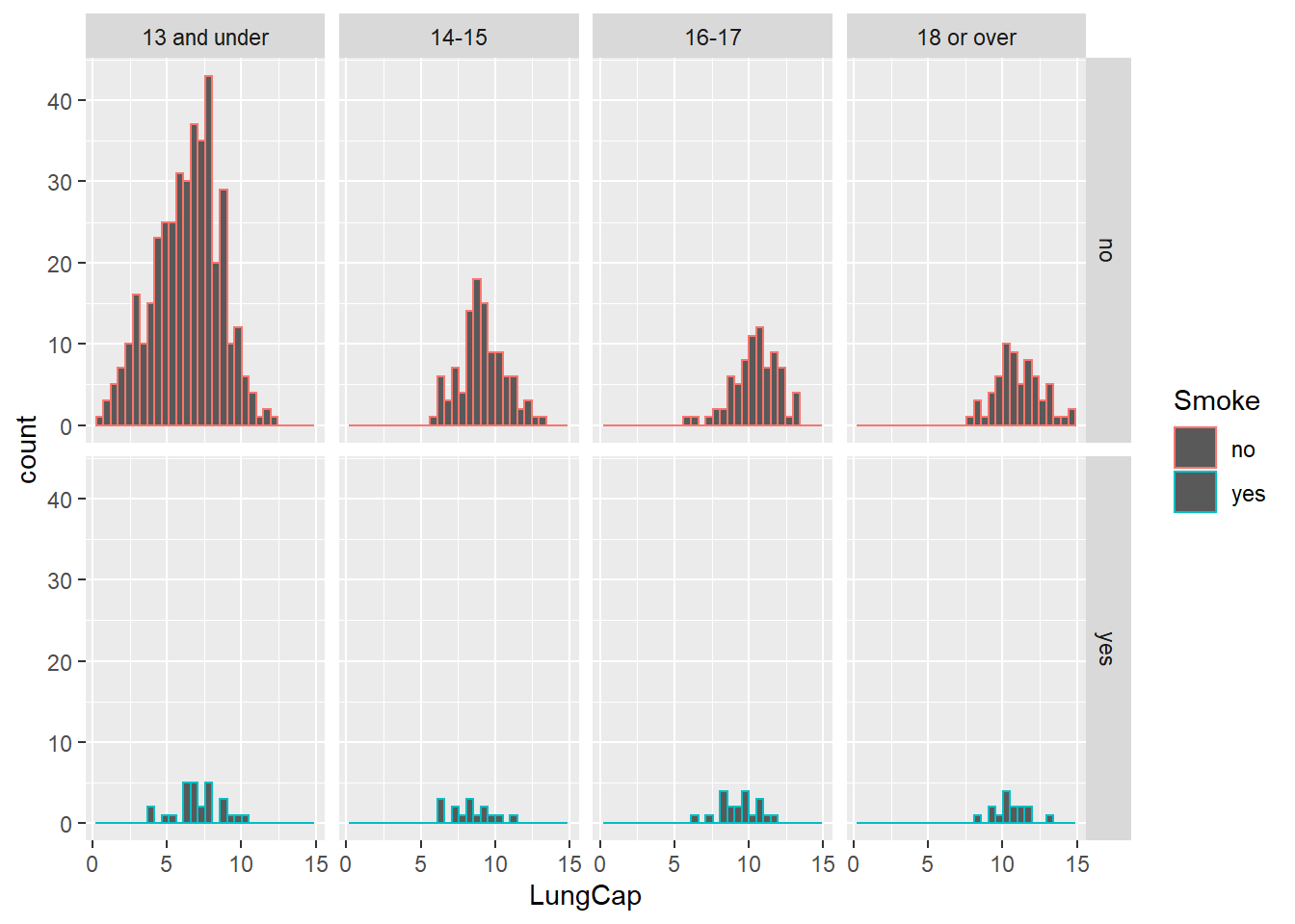
The people who smoke are few in age group of “less than or equal to 13”. From the result we can say age is inversely proportional to the lung capacity.
Form the above data we can say the output are pretty similar that smokers have a lower lung capacity compared to non-smokers
correlation and covariance between lung capacity and age
Covariance is positive and indicates that age and lung capacity are directly related. Correlation is also positive,from these results we can conclude that the lung capacity increases with age.
Warning: `data_frame()` was deprecated in tibble 1.1.0.
Please use `tibble()` instead.# A tibble: 5 × 2
x freq
<int> <dbl>
1 0 128
2 1 434
3 2 160
4 3 64
5 4 24Probability of exactly 2 is 19.75%
Probability that a randomly selected inmate has fewer than 2 prior convictions : 69.38%
The probability that a randomly selected inmate has 2 or fewer prior convictions : 89.13%
The probability that a randomly selected inmate has more than 2 prior convictions? : 10.86%
The expected value for the number of prior convictions : 1.28
The variance is 0.857 and the standard deviation is 0.925
---
title: "HW1"
author: "Niyati Sharma"
desription: "The first homework on descriptive statistics and probability"
date: "10/03/2022"
format:
html:
toc: true
code-fold: true
code-copy: true
code-tools: true
categories:
- hw1
- Niyati Sharma
- desriptive statistics
- probability
---
```{r}
#| label: setup
#| warning: false
library(tidyverse)
library(readxl)
library(ggplot2)
library(stats)
knitr::opts_chunk$set(echo = TRUE)
```
## Question 1
## Read the data from xls file
```{r}
RE <- read_excel("_data/LungCapData.xls")
RE
```
##A
```{r}
RE %>%
  ggplot(aes(LungCap))+
  geom_histogram(bins=20)
```
The histogram looks close to normal distributed.
## B
```{r}
RE %>%
  ggplot(aes (LungCap, color=Gender)) +
  geom_boxplot() +
  theme_classic()
```
The probability density of the female is higher than the males.
## C
```{r}
Mean_Smoker <- RE %>%
  group_by(Smoke) %>%
  summarise(mean = mean(LungCap))
Mean_Smoker
ggplot(RE, aes(LungCap,Smoke))+
  geom_boxplot()
```
From this sample, it appears that smokers have a higher mean lung capacity than non-smokers.
## D
```{r}
RE<-RE %>%
  mutate(Category = as.factor(case_when(Age <= 13 ~ "13 and under",
                           Age == 14 |Age ==15 ~ "14-15",
                           Age == 16 | Age==17 ~ "16-17",
                           Age >= 18 ~ "18 or over"
                           )))
RE
RE %>%
  ggplot(aes( LungCap, color = Smoke)) +
  geom_histogram()+
  facet_grid(Smoke ~ Category)
```
The people who smoke are few in age group of "less than or equal to 13".
From the result we can say age is inversely proportional to the lung capacity.
## E
Form the above data we can say the output are pretty similar that smokers have a lower lung capacity compared to non-smokers
## F
correlation and covariance between lung capacity and age
```{r}
cov(RE$LungCap,RE$Age)
cor(RE$LungCap,RE$Age)
```
Covariance is positive and indicates that age and lung capacity are directly related.
Correlation is also positive,from these results we can conclude that the lung capacity increases with age.
## Question 2
```{r}
x <- c(0:4)
freq <- c(128, 434, 160, 64, 24)
convictions <- data_frame(x, freq)
convictions
```
```{r}
convictions <- convictions %>% mutate(probability = freq/sum(freq))
convictions
```
## A
Probability of exactly 2 is 19.75%
## B
```{r}
a <-head(convictions,2)
sum(a$probability)
```
Probability that a randomly selected inmate has fewer than 2 prior
convictions : 69.38%
## C
```{r}
a <-head(convictions,3)
sum(a$probability)
```
The probability that a randomly selected inmate has 2 or fewer prior
convictions : 89.13%
## D
```{r}
a <-tail(convictions,2)
sum(a$probability)
```
The probability that a randomly selected inmate has more than 2 prior
convictions? : 10.86%
## E
```{r}
WE <- weighted.mean(convictions$x,convictions$probability)
WE
```
The expected value for the number of prior convictions : 1.28
## F
The variance is 0.857 and the standard deviation is 0.925
```{r}
AB <- (sum(freq*((x-WE)^2)))/(sum(freq)-1)
AB
sqrt(AB)
```