Code
library(tidyverse)
library(readxl)
library(ggplot2)
library(stats)

knitr::opts_chunk$set(echo = TRUE)Rahul Gundeti
October 2, 2022
The Lung Capacity data contains 725 rows and 6 columns that determine age, height etc., The key classification parameter is based on smoker vs non-smoker.
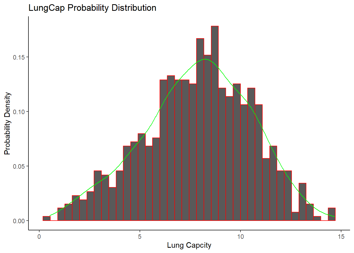
The distribution of LungCap looks as follows:

The observations plotted by histogram are closer to mean which suggests that it is a normal distribution.
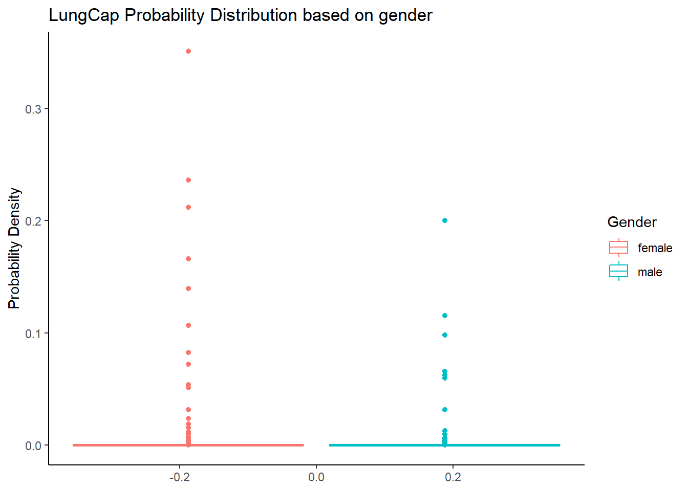
The distribution of LungCap on basis of gender looks as follows:

The box plot shows that the probability density of the male < female.
Comparison of mean lung capacities between smokers and non-smokers:
The table contains the mean lung capacity. The observations suggest that the mean value is higher for smokers than non-smokers. This isn’t entirely correct as the individual biological factors plays a main role. So the data is inadequate to form an opinion.
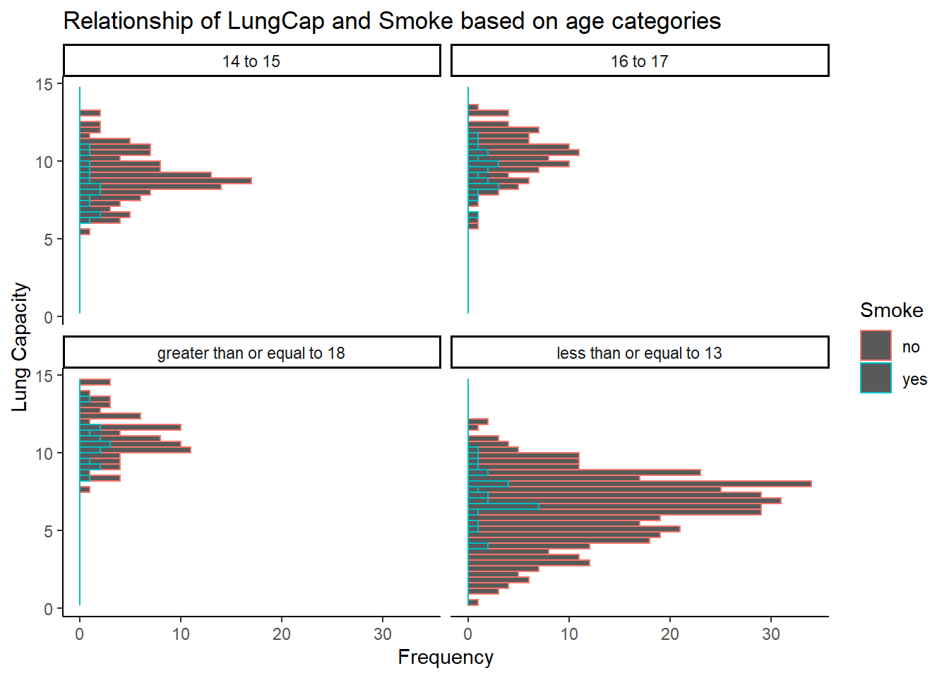
Relationship between Smoke and Lung capacity on basis of given age categories:
lung <- mutate(lung, AgeGrp = case_when(Age <= 13 ~ "less than or equal to 13",
Age == 14 | Age == 15 ~ "14 to 15",
Age == 16 | Age == 17 ~ "16 to 17",
Age >= 18 ~ "greater than or equal to 18"))
lung %>%
ggplot(aes(y = LungCap, color = Smoke)) +
geom_histogram(bins = 40) +
facet_wrap(vars(AgeGrp)) +
theme_classic() +
labs(title = "Relationship of LungCap and Smoke based on age categories", y = "Lung Capacity", x = "Frequency")
From the above plot, we can derive two important observations: 1. The lung capacity of non-smokers is more than smokers. 2. The people who smoke are less in age group of “less than or equal to 13”. So as the result as age increases the lung capacity decreases.
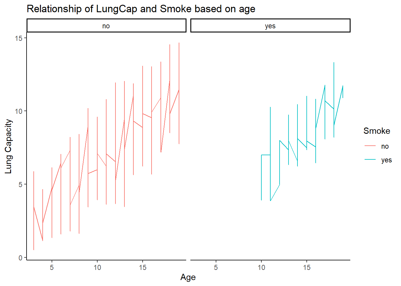
Relationship between Smoke and Lung capacity on basis of age:

Comparing 1_D and 1_E we can find similarity which points that only 10 and above age group smoke.
Calculating the correlation and covariance between Lung Capacity and Age:
[1] 8.738289[1] 0.8196749The comparison shows that the covariance is positive, indicating that lung capacity and age have a direct relationship. As a result, they are moving in the same direction due to the positive correlation as well. This means that as age increases, lung capacity increases as well, which means they are directly proportional.
Warning: `data_frame()` was deprecated in tibble 1.1.0.
Please use `tibble()` instead.
This warning is displayed once every 8 hours.
Call `lifecycle::last_lifecycle_warnings()` to see where this warning was generated.Probability that a randomly selected inmate has exactly 2 prior convictions:
Probability that a randomly selected inmate has fewer than 2 convictions:
Probability that a randomly selected inmate has 2 or fewer prior convictions:
Probability that a randomly selected inmate has more than 2 prior convictions:
Expected value for the number of prior convictions:
Variance for the Prior Convictions:
standard deviation for the Prior Convictions:
---
title: "DACSS603_HW1"
author: "Rahul Gundeti"
description: "Descriptive Statistics and Probability functions"
date: "10/2/2022"
format:
html:
df-print: paged
css: styles.css
toc: true
code-fold: true
code-copy: true
code-tools: true
categories:
- hw1
- desriptive statistics
- probability
---
```{r}
#| label: setup
#| warning: false
library(tidyverse)
library(readxl)
library(ggplot2)
library(stats)
knitr::opts_chunk$set(echo = TRUE)
```
## Question 1
## Reading data
```{r}
lung <- read_excel("C:/Users/gunde/Downloads/LungCapData.xls")
lung
```
The Lung Capacity data contains 725 rows and 6 columns that determine age, height etc., The key classification parameter is based on smoker vs non-smoker.
## 1_A
The distribution of LungCap looks as follows:
```{r}
lung %>%
  ggplot(aes(LungCap, ..density..)) +
  geom_histogram(bins= 40, color = "red") +
  geom_density(color = "green") +
  theme_classic() +
  labs(title = "LungCap Probability Distribution", x = "Lung Capcity", y = "Probability Density")
```
The observations plotted by histogram are closer to mean which suggests that it is a normal distribution.
## 1_B
The distribution of LungCap on basis of gender looks as follows:
```{r}
lung %>%
  ggplot(aes(y = dnorm(LungCap), color = Gender)) +
  geom_boxplot() +
  theme_classic() +
  labs(title = "LungCap Probability Distribution based on gender", y = "Probability Density")
```
The box plot shows that the probability density of the male < female.
## 1_C
Comparison of mean lung capacities between smokers and non-smokers:
```{r}
Mean_smoke <- lung %>%
  group_by(Smoke) %>%
  summarise(mean = mean(LungCap))
Mean_smoke
```
The table contains the mean lung capacity. The observations suggest that the mean value is higher for smokers than non-smokers. This isn't entirely correct as the individual biological factors plays a main role. So the data is inadequate to form an opinion.
## 1_D
Relationship between Smoke and Lung capacity on basis of given age categories:
```{r}
lung <- mutate(lung, AgeGrp = case_when(Age <= 13 ~ "less than or equal to 13",
                                    Age == 14 | Age == 15 ~ "14 to 15",
                                    Age == 16 | Age == 17 ~ "16 to 17",
                                    Age >= 18 ~ "greater than or equal to 18"))

lung %>%
  ggplot(aes(y = LungCap, color = Smoke)) +
  geom_histogram(bins = 40) +
  facet_wrap(vars(AgeGrp)) +
  theme_classic() +
  labs(title = "Relationship of LungCap and Smoke based on age categories", y = "Lung Capacity", x = "Frequency")
```
From the above plot, we can derive two important observations:
1. The lung capacity of non-smokers is more than smokers.
2. The people who smoke are less in age group of "less than or equal to 13".
So as the result as age increases the lung capacity decreases.
## 1_E
Relationship between Smoke and Lung capacity on basis of age:
```{r}
lung %>%
  ggplot(aes(x = Age, y = LungCap, color = Smoke)) +
  geom_line() +
  theme_classic() +
  facet_wrap(vars(Smoke)) +
  labs(title = "Relationship of LungCap and Smoke based on age", y = "Lung Capacity", x = "Age")
```
Comparing 1_D and 1_E we can find similarity which points that only 10 and above age group smoke.
## 1_F
Calculating the correlation and covariance between Lung Capacity and Age:
```{r}
Covariance <- cov(lung$LungCap, lung$Age)
Correlation <- cor(lung$LungCap, lung$Age)
Covariance
Correlation
```
The comparison shows that the covariance is positive, indicating that lung capacity and age have a direct relationship. As a result, they are moving in the same direction due to the positive correlation as well. This means that as age increases, lung capacity increases as well, which means they are directly proportional.
## Question 2
## Reading the table
```{r}
Prior_convitions <- c(0:4)
Inmate_count <- c(128, 434, 160, 64, 24)
prior <- data_frame(Prior_convitions, Inmate_count)
prior
```
```{r}
prior <- mutate(prior, Probability = Inmate_count/sum(Inmate_count))
prior
```
## 2_A
Probability that a randomly selected inmate has exactly 2 prior convictions:
```{r}
prior %>%
  filter(Prior_convitions == 2) %>%
  select(Probability)
```
## 2_B
Probability that a randomly selected inmate has fewer than 2 convictions:
```{r}
random <- prior %>%
  filter(Prior_convitions < 2)
sum(random$Probability)
```
## 2_C
Probability that a randomly selected inmate has 2 or fewer prior convictions:
```{r}
random <- prior %>%
  filter(Prior_convitions <= 2)
sum(random$Probability)
```
## 2_D
Probability that a randomly selected inmate has more than 2 prior convictions:
```{r}
random <- prior %>%
  filter(Prior_convitions > 2)
sum(random$Probability)
```
## 2_E
Expected value for the number of prior convictions:
```{r}
prior <- mutate(prior, Wm = Prior_convitions*Probability)
ev <- sum(prior$Wm)
ev
```
## 2_F
Variance for the Prior Convictions:
```{r}
variance <-sum(((prior$Prior_convitions-ev)^2)*prior$Probability)
variance
```
standard deviation for the Prior Convictions:
```{r}
sqrt(variance)
```