Final Project: Part 2 (Update)

Florida Homelessness by County 2018-2020

finalpart2

shelton

homelessness

Author

Dane Shelton

Published

November 12, 2022

Homelessness in Florida

Homelessness is a complex living situation with several qualifying conditions; at its most simple state, the U.S Dept. of Housing and Urban Development defines it as lacking a fixed, regular nighttime residence (not a shelter) or having a nighttime residence not designed for human accommodation¹.

On a single night in 2020, over 500,000² people experienced homelessness in the United States. Florida, with the third largest state population , had the fourth largest homeless population of 2020 with 27,487².

Florida counties represent a large age range and varying demographic profiles; the state is a hub to a variety of industries including tourism, defense, agriculture, and information technology. Investigating homelessness in Florida counties with robust data can lead to several conclusions about who is being impacted where, and how state policy is failing groups of a diverse population.

Carole Zugazaga’s 2004 study of 54 single homeless men, 54 single homeless women, and 54 homeless women with children in the Central Florida area investigated stressful life events common among homeless people. The interviews revealed that women were more likely to have been sexually or physically assaulted, while men were more likely to have been incarcerated or abuse drugs/alcohol. Homeless women with children were more likely to be in foster care as a youth.

Nearly a decade later,county-level data can be used to investigate the relationship between Zugazaga’s reported stressful life events (incarceration, drug arrests, poverty, forcible sex…)³ and homelessness counts.

Research Question

Do particular life stressors increase a population’s vulnerability to homelessness?

Homelessness is not a new issue in the United States, yet homeless policy targets elimination via criminalization rather than prevention. Despite state and federal governments being aware of the circumstances that increase vulnerability to homelessness for decades, I anticipate all of the variables to remain significant in a model relating stressors to Florida homelessness counts 2018-2020.

Research Hypothesis

H₀: All stressors are insignificant in predicting homelessness counts ( B_i = 0 for i=0,1,2,…n )

H_A: At least one stressor B_i is significant in predicting homelessness counts

The data florida_1820.csv⁴ describes population, homelessness counts, poverty counts and several other demographic indicators³ at the county level for 2018-2020. All 67 Florida counties have observations for the 3 years giving us 201 observations of 15 variables. Each observation provides a count of each variables from a single county for a year within 2018-2020.

The data were collected from the Florida Department of Health. Variable names³ were used as search indicators to produce counts for Florida counties. Unfortunately, we cannot accurately analyze the effect of COVID-19 as data is incomplete for the majority of counties in 2021.

Intro to Data

    County               Year      Homeless (Count)   Population     
 Length:201         Min.   :2018   Min.   :   0.0   Min.   :   8367  
 Class :character   1st Qu.:2018   1st Qu.:  11.0   1st Qu.:  28089  
 Mode  :character   Median :2019   Median : 151.0   Median : 130642  
                    Mean   :2019   Mean   : 427.8   Mean   : 317746  
                    3rd Qu.:2020   3rd Qu.: 563.0   3rd Qu.: 367471  
                    Max.   :2020   Max.   :3516.0   Max.   :2864600  
                                                                     
 Unemployment Rate   Median Inc    Incarceration (Rateper1000) Poverty (Count) 
 Min.   : 2.100    Min.   :34583   Min.   : 0.60               Min.   :   906  
 1st Qu.: 3.400    1st Qu.:41401   1st Qu.: 2.50               1st Qu.:  4901  
 Median : 4.000    Median :50640   Median : 3.40               Median : 16210  
 Mean   : 4.697    Mean   :51116   Mean   : 3.84               Mean   : 42922  
 3rd Qu.: 5.600    3rd Qu.:58093   3rd Qu.: 4.50               3rd Qu.: 46034  
 Max.   :13.500    Max.   :83803   Max.   :18.60               Max.   :482656  
                                                                               
 Drug Arrests (Count) Relocated (Rate) Sub Abuse Enrollment (Count)
 Min.   :   13        Min.   : 4.689   Min.   :   5.0              
 1st Qu.:  225        1st Qu.:11.244   1st Qu.:  76.0              
 Median :  729        Median :12.700   Median : 250.0              
 Mean   : 1558        Mean   :13.288   Mean   : 877.6              
 3rd Qu.: 1903        3rd Qu.:14.544   3rd Qu.:1030.0              
 Max.   :13038        Max.   :22.553   Max.   :6272.0              
                                                                   
 Adult Psych Beds (Count) Severe Housing Problems (Rate) Forcible Sex (Count)
 Min.   :  0.00           Min.   : 9.6                   Min.   :   0.0      
 1st Qu.:  0.00           1st Qu.:13.3                   1st Qu.:  14.0      
 Median :  0.00           Median :15.4                   Median :  45.0      
 Mean   : 66.26           Mean   :15.8                   Mean   : 170.5      
 3rd Qu.: 84.00           3rd Qu.:17.3                   3rd Qu.: 225.0      
 Max.   :778.00           Max.   :29.8                   Max.   :1408.0      
                          NA's   :134                                        
 Foster Care (Count)
 Min.   :   3.0     
 1st Qu.:  33.0     
 Median : 153.0     
 Mean   : 326.1     
 3rd Qu.: 353.0     
 Max.   :2289.0

COMMENT PLOTS TAB

Expanding Intro to Data exposes summary statistics including mean, range, quantiles, and standard deviation for all 15 variables. The table below the summaries provides arranged figures for basic parameters of interest grouped by county.

LATER: Plots, Isolate more variables of interest with grouping, group by year?

on Assumption of Validity

While over 10 variables are predicting Homeless (Rate) across Florida counties, there are still limitations when attempting to comment on the magnitude of an individual stressor. Stressors influence homelessness by driving those in severe situations out of their home or away from their place of origin. Homeless (Rate) is not an ideal measure of magnitude as the homeless population migrating to escape or avoid certain stressors would result in counties with low stressor values having a higher homeless population; this effect is left unexplained by the following models.

The variable Relocated (Rate) is included as an attempt to control for new movement, however this doesn’t completely capture county-to-county migration.
FL Charts has data that records Population Who Lived in a Different County One Year Earlier, however with the data spanning 2009-2014, using values recorded 4 years prior to our data isn’t desirable either.
The most appropriate data to accurately capture county-to-county migration is here via the US Census Bureau. The -In, -Out, -Net... spreadsheet provides totals for each county in the United States and movement to all other US counties; unfortunately, this data is too complex to wrangle into the simple data set florida_1820.csv.

on Assumption of Linearity

Code

# Fit 1: A Linear Regression Model With All Vars

# Checking Linearity of variables not supported by our literature

florida_matrix <- florida_og_rates %>%
                    select(-c('County', 
                              'Year', 
                              'Poverty (Rate)', 
                              'Severe Housing Problems (Rate)',
                              'Sub Abuse Enrollment (Rate)',
                              'Drug Arrests (Rate)',
                              'Adult Psych Beds (Rate)',
                              'Foster Care (Rate)',
                              'Forcible Sex (Rate)' ))%>%
                      pairs()

Code

florida_matrix

NULL

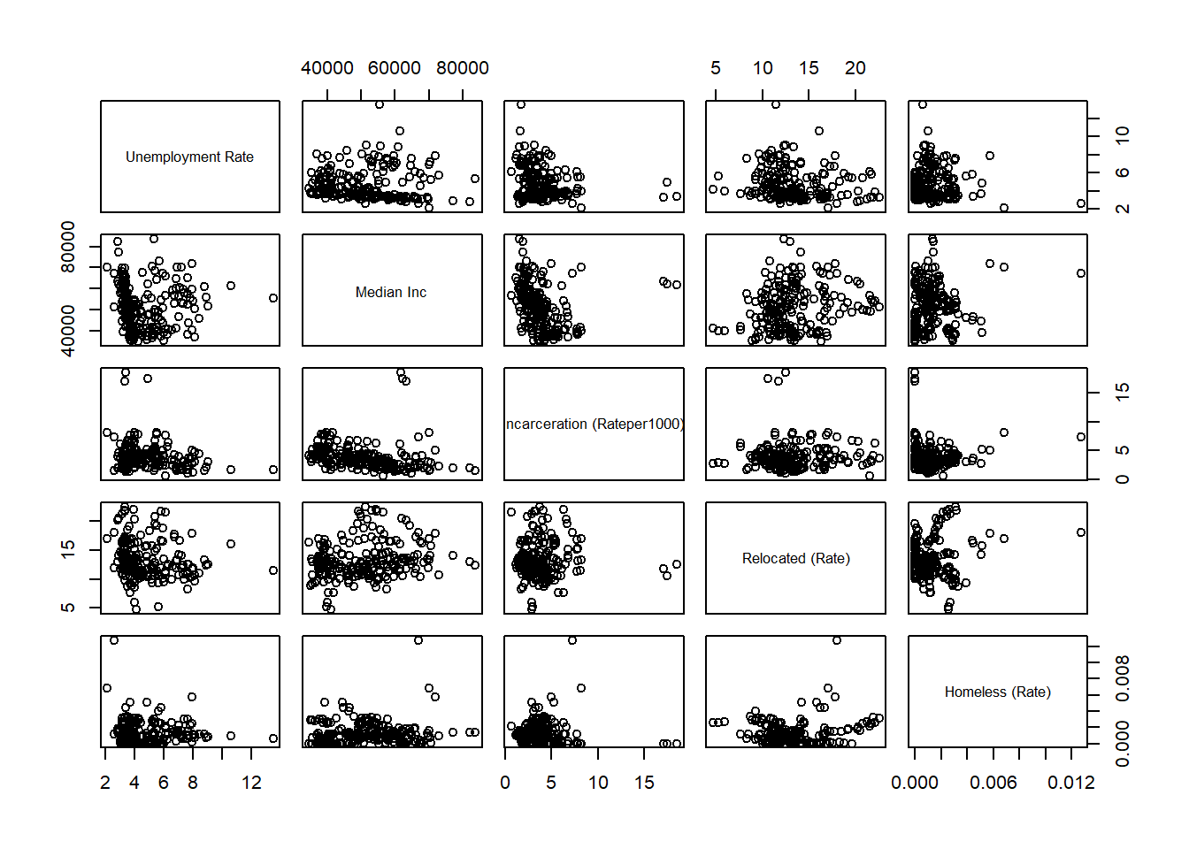
A quick look at variables with a relationship to homelessness not mentioned in Zugazaga’s study, or those that needed further investigation are shown here to confirm that while the associations are weak, a linear approximation is appropriate.

Linear Regression Models

Fit 1: All Variables (No Transformations)

Code

# Linear relationship appears appropriate for all, possibly attempt log transformation on UE Rate?

# Creating A Linear Model with all variables included: No Transformations

# County Removed as too many levels; improvement: NWFL, NFL, CFL, SWFL, SOFLO categories?

fit1 <- florida_og_rates %>% 
          select(-'County')%>%
            
            lm(formula=`Homeless (Rate)` ~.)

summary(fit1)


Call:
lm(formula = `Homeless (Rate)` ~ ., data = .)

Residuals:
       Min         1Q     Median         3Q        Max 
-0.0021639 -0.0008741 -0.0002945  0.0003981  0.0078061 

Coefficients: (1 not defined because of singularities)
                                   Estimate Std. Error t value Pr(>|t|)  
(Intercept)                      -5.014e-03  3.408e-03  -1.471   0.1469  
Year                                     NA         NA      NA       NA  
`Unemployment Rate`              -1.993e-04  4.062e-04  -0.491   0.6257  
`Median Inc`                      5.022e-08  3.506e-08   1.433   0.1576  
`Incarceration (Rateper1000)`     3.479e-05  1.009e-04   0.345   0.7316  
`Relocated (Rate)`               -6.075e-05  7.624e-05  -0.797   0.4290  
`Severe Housing Problems (Rate)`  1.584e-04  7.639e-05   2.074   0.0428 *
`Poverty (Rate)`                  4.429e-03  8.195e-03   0.540   0.5911  
`Drug Arrests (Rate)`             9.809e-02  7.369e-02   1.331   0.1886  
`Sub Abuse Enrollment (Rate)`     4.671e-02  1.374e-01   0.340   0.7351  
`Adult Psych Beds (Rate)`         3.177e+00  2.138e+00   1.486   0.1429  
`Forcible Sex (Rate)`             3.717e-02  1.093e+00   0.034   0.9730  
`Foster Care (Rate)`              6.768e-01  3.664e-01   1.847   0.0701 .
---
Signif. codes:  0 '***' 0.001 '**' 0.01 '*' 0.05 '.' 0.1 ' ' 1

Residual standard error: 0.00157 on 55 degrees of freedom
  (134 observations deleted due to missingness)
Multiple R-squared:  0.3441,    Adjusted R-squared:  0.2129 
F-statistic: 2.623 on 11 and 55 DF,  p-value: 0.00914

Code

rss1 <- deviance(fit1)
print(c('RSS Fit 1', rss1))

[1] "RSS Fit 1"            "0.000135542075603397"

The first model predicts Homeless (Rate) using all variables, without any transformations or interactions. This causes 134 observations to removed as they are missing values for Severe Housing Problems (Rate).
Only 1 variable is deemed significant at alpha = 0.05; those without a star (see output) are deemed inconsequential in predicting Homeless (Rate) by this model.
We see the effect of Relocated (Rate) is negative indicating that migration can have a negative impact on homelessness by county, as mentioned in ‘Assumptions on Validity’ (above)
Looking at the signs and amgnitude of the predicted (insignificant) variables, they seem plausible - Increases in variables like Drug Arrests (Rate) or Poverty (Rate) decreases homelessness? It is clear the movement confounder mentioned above is influencing results. Select transformations or interactions could quell issues.

Fit 1: Diagnostics

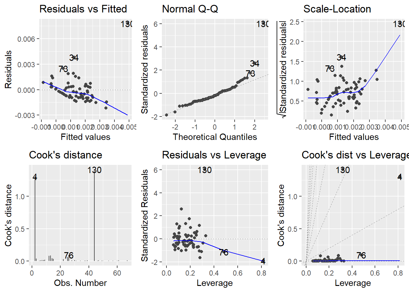
Fit 1 does a poor job of obeying the assumptions regarding residuals of linear regression.
Residuals vs Fitted shows the residuals increasing in size the greater the fitted value is, violating the linearity and independence assumption.
As for residuals following an approximately normal distribution, the Q-Q Plot shows a noticeable deviation from the diagonal.
There are several points that could be considered outliers due to their residual or leverage value, how greatly they influence the points around them in the model.
- Observations 16, 37, and 154 represent Miami-Dade and Broward County - two of the largest and most urbanized regions in the state. Pinellas County (154) is a top 10 county in terms of population.
- Monroe County (130) has large positive residuals, indicating our model greatly under-estimated the number of homeless people in this county.

Fit 2: All Variables + Interactions + Transformations + Fill all Observations

Code

fit2 <- florida_og %>% 
          select(-c('County','Year'))%>%
            mutate(`Unemployment Rate` = log(`Unemployment Rate`),
                   `Incarceration (Rateper1000)` = log(`Incarceration (Rateper1000)`))%>%
              fill('Severe Housing Problems (Rate)', .direction="down")%>%
                
                lm(formula=`Homeless (Rate)` ~ . 
                   + `Unemployment Rate`* `Population`
                   + `Poverty (Rate)`* `Median Inc`)

Error in eval(predvars, data, env): object 'Homeless (Rate)' not found

Code

summary(fit2)

Error in h(simpleError(msg, call)): error in evaluating the argument 'object' in selecting a method for function 'summary': object 'fit2' not found

Code

bic2 <- BIC(fit2)

Error in BIC(fit2): object 'fit2' not found

Code

print(c('BIC Fit 2:', bic2))

Error in print(c("BIC Fit 2:", bic2)): object 'bic2' not found

Code

rss2 <- deviance(fit2)

Error in deviance(fit2): object 'fit2' not found

Code

print(c('RSS Fit 2', rss2))

Error in print(c("RSS Fit 2", rss2)): object 'rss2' not found

In Fit 2, the values from Severe Housing Problems (Rate) were filled down provide values to restore all observations for use in the regression.
Both Unemployment Rate and Incarceration Rate were log() transformed to improve linearity with the outcome. Two interaction terms were included.

Fit 2: Diagnostics

Error in autoplot(fit2, 1:6, ncol = 3): object 'fit2' not found

Error in eval(expr, envir, enclos): object 'diag2' not found

The appearance of the diagnostic plots improved greatly after the mentioned transformations, with only the Q-Q Plot remaining the same.
We still see the influence from the larger counties in the leverage plots. Observation 108, Lee - another high population county, is over-estimated by the model.
- All in Southern Florida, Lee County differs from Broward or Miami-Dade in that it is home to a slightly older population; this may explain the over-estimate.

Fit 3: Partial Model - Preferred Variables

Code

fit3 <- florida_og %>% 
          select(-'County')%>%
            mutate(`Incarceration (Rateper1000)` = log(`Incarceration (Rateper1000)`))%>%
            #mutate(`Unemployment Rate` = log(`Unemployment Rate`))%>%
                
                lm(formula=`Homeless (Rate)` ~ 
                   `Poverty (Rate)`
                   + `Median Inc`
                   + `Incarceration (Rateper1000)`
                   #+ `Severe Housing Problems (Rate)`
                   + `Relocated (Rate)`
                   + `Drug Arrests (Rate)`
                   + `Adult Psych Beds (Rate)`
                   + `Forcible Sex (Rate)`
                   + `Foster Care (Rate)`
                   + `Poverty (Rate)`* `Median Inc`)

Error in eval(predvars, data, env): object 'Homeless (Rate)' not found

Code

summary(fit3)

Error in h(simpleError(msg, call)): error in evaluating the argument 'object' in selecting a method for function 'summary': object 'fit3' not found

Code

bic3 <- BIC(fit3)

Error in BIC(fit3): object 'fit3' not found

Code

print(c('BIC Fit 3:', bic3))

Error in print(c("BIC Fit 3:", bic3)): object 'bic3' not found

Code

rss3 <- deviance(fit3)

Error in deviance(fit3): object 'fit3' not found

Code

print(c('RSS Fit 3', rss3))

Error in print(c("RSS Fit 3", rss3)): object 'rss3' not found

A model containing just variables I believed would provide the best fit.

Fit 3: Diagnostics

Error in autoplot(fit3, 1:6, ncol = 3): object 'fit3' not found

Error in eval(expr, envir, enclos): object 'diag3' not found

The diagnostic plots of this model leave much to be desired, similarly to Fit 1

Model Selection

Comparing Residuals Sum Squared, R^2, and BIC to evaluate Fit 2 versus Fit 3, I would select Fit 2 for both prediction and inference. Using all values, including interactions, and a log transformation results in the lowest RSS and BIC, and maximizes the Adjusted R-Squared. It provides the most appropriate diagnostic plots.

Interaction terms: Population:Unemployment Rate and Median Income:Poverty (Rate)

I assumed the influence of the unemployment rate would change at different population values. A small unemployment rate of 2% will not have the same effect on the outcome in a county of 100,000 as a 2% rate in a county of 2.5 million.
Our model found the impact of Unemployment Rate when predicting homelessness in a county diminished as Population increased.
When considering the number of people living below the poverty line, it’s reasonable to believe the influence of number of citizens living below the poverty line will have a greater impact on homelessness in counties with lower median incomes.
Another negative slope, the model found the impact of Median Inc to decrease (taking it below zero) as Poverty (Rate) increases.

Research Question:

Using all of the values rather than just 2019 not only improves Residual Standard Error and Adjusted R-Squared value, it corrects the signs and magnitude of effects. Several more stressors were deemed significant at the 0.05 and 0.10 level.
All of Zugazaga’s effects had the correct sign demonstrating their influence in this model, but only Foster Care and Drug Arrests were significant at the 0.05 level as hypothesized. This significance is a comment on the mathematical properties of the model rather than on the real-life influence of the stressors. Incarceration and Forcible Sex are influential situations that can contribute to homelessness.
Drug Arrests again has a negative slope, a concerning suggestion would be incarceration as a form of drug abuse intervention is decreasing homelessness; however, Incarceration Rate has a large positive slope, dispelling this notion.
- This result speaks more to recidivism rates in Florida’s communities as well as the challenge that is reintegrating into society after release. The negative slope still indicates drug abuse has a role in increasing homeless in Florida counties.

Was the Research Question Answered?

As hypothesized, the model proved several stressors to be significant in predicting Homeless Rates across Florida
Unfortunately, the study is unable to make a substantial comment on which stressors most increased vulnerability to Homelessness, evaluating magnitude. To do this, deeper demographic variables would need to be included, as well as controlling for stressors as a push factor in homeless migration.

Prediction vs Inference

The goal of this brief study was to make inferences regarding stressors’ impact on Homelessness (Rates) in Florida.
If prediction was our focus, I would use new 2021 data from FL Charts without the Homeless (Rate) column to test the efficacy of Fit 2 as a predictive tool.

While the data is great illustration of homelessness in Florida by county, there are improvements that could be made to both data collection and the research question itself to further the study.

Data:

Unfortunately, FL Health Charts did not provide demographic breakdown for the homeless population (Age, Sex, Race), which would drastically widen the scope of the analysis, leading to far more interesting conclusions.
There is only have data for a three year period; this is too small of a range to make a strong statement about the impact of homeless policy on Florida counties or how the relevance of certain stressors has changed over time. For a more in depth study I would begin with a 10 year range.

Research Question:

Demographic breakdown of stressors’ impact (Age, Sex, Race)
Extend the question to the entire country, providing a breakdown by state
Compare to foreign countries to contrast governments’ approaches to homelessness and leading causes of homelessness around the world.

Variable Definitions and Collection Methods here

Carol Zugazaga R4DS LSR R packages?

Footnotes

_{1.) Homeless Definition}

_{2.) US Interagency Council on Homelessness}

_{3.) Explanation of variables and collection method in Codebook tab}