Code
library(tidyverse)
library(readr)
library(stringr)
library(dplyr)
library(hrbrthemes)

knitr::opts_chunk$set(echo = TRUE, warning=FALSE, message=FALSE)library(tidyverse)
library(readr)
library(stringr)
library(dplyr)
library(hrbrthemes)
knitr::opts_chunk$set(echo = TRUE, warning=FALSE, message=FALSE)There are two main types of safety concerns for any living species on earth. One is natural calamities which are obviously uncontrollable, and the second is man-made. The man-made safety related problems can be reduced or controlled if we study it properly and take actions accordingly. Among the man- made safety issues, crimes are always on the top of the list. The study of crime data will give us insights on how to not be a victim, by choosing a place that is less prone to a crime activities. So I decided to take the crime dataset of Massachusetts state and study on it to see if a person chooses to be in a particular location in a county at a specific time of the day, whether it will be safe or not. I am trying to compare the numbers of different counties in the state.
This is a study on crime data of Massachusetts states. The dataset is a county based number of crimes at a location at a specific time of the day. The data is been taken from the public website of police department. Eventhough the data can be downloaded for the past years, I decided to take the data for 2021 as it is the most recent data. The data from police department had only the number of crimes at a location at a time of the day. If we take just the number of crime as such without considering other factors like the population or population density of the county, the analysis will be incomplete. So as an initial study, I decided to take the county-wise population data from the census 2020 and do the study on crime data as a function relative to the population of the county of occurance.
As there are 14 counties in Massachusetts, my data contains 14 separate county files to be read along with the population data of Massachusetts counties.
ma_population <- read_csv('_data/601_final_project_jerin_jacob/MA_population.csv', col_names = c("Number", "County", "Population"))
ma_population$County <- word(ma_population$County, 1)
ma_population <- ma_population[ -c(1) ]
ma_population
# A tibble: 14 × 2
County Population
<chr> <dbl>
1 Middlesex 1605899
2 Worcester 826655
3 Suffolk 801162
4 Essex 787038
5 Norfolk 703740
6 Bristol 563301
7 Plymouth 518597
8 Hampden 466647
9 Barnstable 213505
10 Hampshire 161361
11 Berkshire 125927
12 Franklin 70529
13 Dukes 17430
14 Nantucket 11212filepath <- "_data/601_final_project_jerin_jacob/"
csv_file_names <- list.files(path = filepath, pattern = "_2021*")
#csv_file_namesread_crimes<-function(file_name){
x<-unlist(str_split(file_name, pattern="[[:punct:]]", n=3))
read_csv(paste0(filepath, file_name),
skip = 8,
col_names = c("Location","6-9pm","9-12pm","12-3am","3-6am","6-9am","9-12noon","12-3pm","3-6pm"))%>%
mutate(County = x[1],
Year = x[2])
}
counties<-
purrr::map_dfr(csv_file_names, read_crimes)
head(counties)# A tibble: 6 × 11
Locat…¹ `6-9pm` 9-12p…² 12-3a…³ `3-6am` `6-9am` 9-12n…⁴ 12-3p…⁵ `3-6pm` County
<chr> <dbl> <dbl> <dbl> <dbl> <dbl> <dbl> <dbl> <dbl> <chr>
1 All Lo… 969 661 430 190 607 1314 1421 1264 Barns…
2 Reside… 456 314 190 94 287 661 703 629 Barns…
3 Commer… 226 138 96 41 114 243 272 292 Barns…
4 Air/Bu… 3 NA NA NA NA 1 3 2 Barns…
5 Bank/S… 4 2 NA 1 10 12 21 15 Barns…
6 Bar/Ni… 2 11 13 1 2 1 4 4 Barns…
# … with 1 more variable: Year <chr>, and abbreviated variable names ¹Location,
# ²`9-12pm`, ³`12-3am`, ⁴`9-12noon`, ⁵`12-3pm`dim(counties)[1] 756 11The population data is a clean data that has 14 rows of each county and the population.
The crime data contains 54 rows and 11 columns for each county files. 54 rows are different location types in the county categorised as where any crime can possibly occur.
In the dataset, there is a row for ‘All Location Types’. I expected that to be same as the sum of all other Locations but it was not. This could be due to either data entry errors or overlapping/duplication of data in Locations with similar names. I could find 6 such Locations that duplicated. ‘Commercial’, ‘Educational Facility’, ‘Government/Public Building and other’, ‘Road/Parking/Camps’, ‘Field/Woods/Waterways/Camps’ and ‘Construction/Industrial/Farm’. Those 6 Location types are just grouping of two or more other Location Types.
first_county <- counties %>%
  slice(1:54)
first_county
# A tibble: 54 × 11
Location `6-9pm` 9-12p…¹ 12-3a…² `3-6am` `6-9am` 9-12n…³ 12-3p…⁴ `3-6pm`
<chr> <dbl> <dbl> <dbl> <dbl> <dbl> <dbl> <dbl> <dbl>
1 "All Locatio… 969 661 430 190 607 1314 1421 1264
2 "Residence/H… 456 314 190 94 287 661 703 629
3 "Commercial" 226 138 96 41 114 243 272 292
4 "Air/Bus/Tra… 3 NA NA NA NA 1 3 2
5 "Bank/Saving… 4 2 NA 1 10 12 21 15
6 "Bar/Nightcl… 2 11 13 1 2 1 4 4
7 "Commercial/… 37 8 5 2 27 67 44 49
8 "Convenience… 26 14 5 4 7 15 14 22
9 "Department/… 19 1 2 1 6 8 36 38
10 "Drug Store/… 19 9 9 3 13 26 16 19
# … with 44 more rows, 2 more variables: County <chr>, Year <chr>, and
# abbreviated variable names ¹`9-12pm`, ²`12-3am`, ³`9-12noon`, ⁴`12-3pm`first_county2 <- first_county %>%
slice(2:54)
mapply(sum,first_county2[,c(2:9)], na.rm= TRUE) 6-9pm 9-12pm 12-3am 3-6am 6-9am 9-12noon 12-3pm 3-6pm
1406 944 629 271 868 1858 2008 1803 So I checked by droping those overlapping/duplicated locations for the Barnstable County and again rechecked. Now the sum of the locations is same as that of ‘All Location Types’.
dfRemain <- first_county[-c(3, 22,27,42,47,38), ]


dfRemain
# A tibble: 48 × 11
Location `6-9pm` 9-12p…¹ 12-3a…² `3-6am` `6-9am` 9-12n…³ 12-3p…⁴ `3-6pm`
<chr> <dbl> <dbl> <dbl> <dbl> <dbl> <dbl> <dbl> <dbl>
1 "All Locatio… 969 661 430 190 607 1314 1421 1264
2 "Residence/H… 456 314 190 94 287 661 703 629
3 "Air/Bus/Tra… 3 NA NA NA NA 1 3 2
4 "Bank/Saving… 4 2 NA 1 10 12 21 15
5 "Bar/Nightcl… 2 11 13 1 2 1 4 4
6 "Commercial/… 37 8 5 2 27 67 44 49
7 "Convenience… 26 14 5 4 7 15 14 22
8 "Department/… 19 1 2 1 6 8 36 38
9 "Drug Store/… 19 9 9 3 13 26 16 19
10 "Grocery/Sup… 24 3 NA 1 7 26 23 27
# … with 38 more rows, 2 more variables: County <chr>, Year <chr>, and
# abbreviated variable names ¹`9-12pm`, ²`12-3am`, ³`9-12noon`, ⁴`12-3pm`all_location <- dfRemain[c(1), ]
all_location %>%
select(2:9)# A tibble: 1 × 8
`6-9pm` `9-12pm` `12-3am` `3-6am` `6-9am` `9-12noon` `12-3pm` `3-6pm`
<dbl> <dbl> <dbl> <dbl> <dbl> <dbl> <dbl> <dbl>
1 969 661 430 190 607 1314 1421 1264df <- dfRemain[-c(1), ]
mapply(sum,df[,c(2:9)], na.rm= TRUE) 6-9pm 9-12pm 12-3am 3-6am 6-9am 9-12noon 12-3pm 3-6pm
969 661 430 190 607 1314 1421 1264 new_county_data<-subset(counties, Location != 'Commercial' & Location !='Educational Facility' & Location != 'Government/Public Building and other' & Location != 'Road/Parking/Camps' & Location != 'Field/Woods/Waterways/Camps' & Location != 'Construction/Industrial/Farm' & Location != 'All Location Types')
new_county_data# A tibble: 658 × 11
Location `6-9pm` 9-12p…¹ 12-3a…² `3-6am` `6-9am` 9-12n…³ 12-3p…⁴ `3-6pm`
<chr> <dbl> <dbl> <dbl> <dbl> <dbl> <dbl> <dbl> <dbl>
1 "Residence/H… 456 314 190 94 287 661 703 629
2 "Air/Bus/Tra… 3 NA NA NA NA 1 3 2
3 "Bank/Saving… 4 2 NA 1 10 12 21 15
4 "Bar/Nightcl… 2 11 13 1 2 1 4 4
5 "Commercial/… 37 8 5 2 27 67 44 49
6 "Convenience… 26 14 5 4 7 15 14 22
7 "Department/… 19 1 2 1 6 8 36 38
8 "Drug Store/… 19 9 9 3 13 26 16 19
9 "Grocery/Sup… 24 3 NA 1 7 26 23 27
10 "Hotel/Motel… 36 30 18 26 13 31 39 21
# … with 648 more rows, 2 more variables: County <chr>, Year <chr>, and
# abbreviated variable names ¹`9-12pm`, ²`12-3am`, ³`9-12noon`, ⁴`12-3pm`dim(counties)[1] 756 11ma_crime_2021 <- new_county_data %>% left_join(ma_population,by="County")The number of crimes per 1000 people in the county can be a good way to start with the analysis. So I scaled down the population data to per 1000.
crime_per_population <- ma_crime_2021 %>%
    mutate(across(c(2:9),
           .fns = ~./(Population/1000)))
crime_per_population
# A tibble: 658 × 12
Location `6-9pm` `9-12pm` `12-3am` `3-6am` `6-9am` 9-12n…¹ 12-3p…² `3-6pm`
<chr> <dbl> <dbl> <dbl> <dbl> <dbl> <dbl> <dbl> <dbl>
1 "Residen… 2.14 1.47 0.890 0.440 1.34 3.10 3.29 2.95
2 "Air/Bus… 0.0141 NA NA NA NA 0.00468 0.0141 0.00937
3 "Bank/Sa… 0.0187 0.00937 NA 0.00468 0.0468 0.0562 0.0984 0.0703
4 "Bar/Nig… 0.00937 0.0515 0.0609 0.00468 0.00937 0.00468 0.0187 0.0187
5 "Commerc… 0.173 0.0375 0.0234 0.00937 0.126 0.314 0.206 0.230
6 "Conveni… 0.122 0.0656 0.0234 0.0187 0.0328 0.0703 0.0656 0.103
7 "Departm… 0.0890 0.00468 0.00937 0.00468 0.0281 0.0375 0.169 0.178
8 "Drug St… 0.0890 0.0422 0.0422 0.0141 0.0609 0.122 0.0749 0.0890
9 "Grocery… 0.112 0.0141 NA 0.00468 0.0328 0.122 0.108 0.126
10 "Hotel/M… 0.169 0.141 0.0843 0.122 0.0609 0.145 0.183 0.0984
# … with 648 more rows, 3 more variables: County <chr>, Year <chr>,
# Population <dbl>, and abbreviated variable names ¹`9-12noon`, ²`12-3pm`crime_per_population <- pivot_longer(crime_per_population, `6-9pm`:`3-6pm`, names_to = "Time_of_day", values_to = "Crime_rate")df <- crime_per_population[ -c(3,4) ]
head(df)# A tibble: 6 × 4
Location County Time_of_day Crime_rate
<chr> <chr> <chr> <dbl>
1 Residence/Home Barnstable 6-9pm 2.14
2 Residence/Home Barnstable 9-12pm 1.47
3 Residence/Home Barnstable 12-3am 0.890
4 Residence/Home Barnstable 3-6am 0.440
5 Residence/Home Barnstable 6-9am 1.34
6 Residence/Home Barnstable 9-12noon 3.10 summary(df) Location County Time_of_day Crime_rate
Length:5264 Length:5264 Length:5264 Min. :0.0006
Class :character Class :character Class :character 1st Qu.:0.0064
Mode :character Mode :character Mode :character Median :0.0281
Mean :0.1415
3rd Qu.:0.0953
Max. :5.0916
NA's :1970 According to the data, the safest place in Massachusetts is an Air/Bus/Train Terminal in Middlesex at 12-3 am. Apparently, residences of Hampden between 3-6 pm turns out to be the most unsafe place or where most crimes happen.
df[which.max(df$Crime_rate),]# A tibble: 1 × 4
Location County Time_of_day Crime_rate
<chr> <chr> <chr> <dbl>
1 Residence/Home Hampden 3-6pm 5.09df[which.min(df$Crime_rate),]# A tibble: 1 × 4
Location County Time_of_day Crime_rate
<chr> <chr> <chr> <dbl>
1 Air/Bus/Train Terminal Middlesex 12-3am 0.000623Checking whether all locations in Hampden have high crime rates and if Middlesex is safe in all locations.
df_middlesex <- df %>%
  filter(County == "Middlesex")

ggplot(df_middlesex, aes(x=Time_of_day, y=Crime_rate)) +
  geom_segment( aes(x=Time_of_day, xend=Time_of_day, y=0, yend=Crime_rate)) +
geom_point( size=5, color="red", fill=alpha("orange", 0.3), alpha=0.7, shape=21, stroke=2) 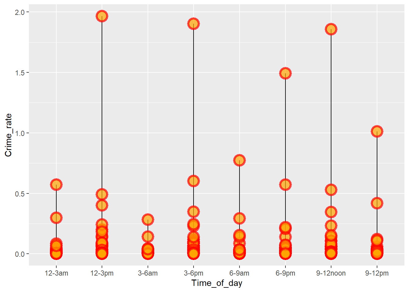
df_hampden <- df %>%
  filter(County == "Hampden")

ggplot(df_hampden, aes(x=Time_of_day, y=Crime_rate)) +
  geom_segment( aes(x=Time_of_day, xend=Time_of_day, y=0, yend=Crime_rate)) +
  geom_point( size=5, color="red", fill=alpha("orange", 0.3), alpha=0.7, shape=21, stroke=2)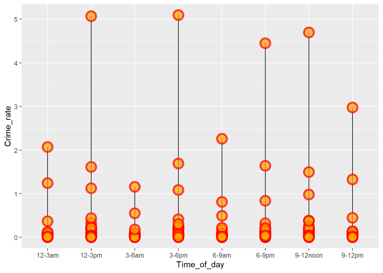
df %>% ggplot(aes(Time_of_day, Crime_rate, color=County)) + geom_point()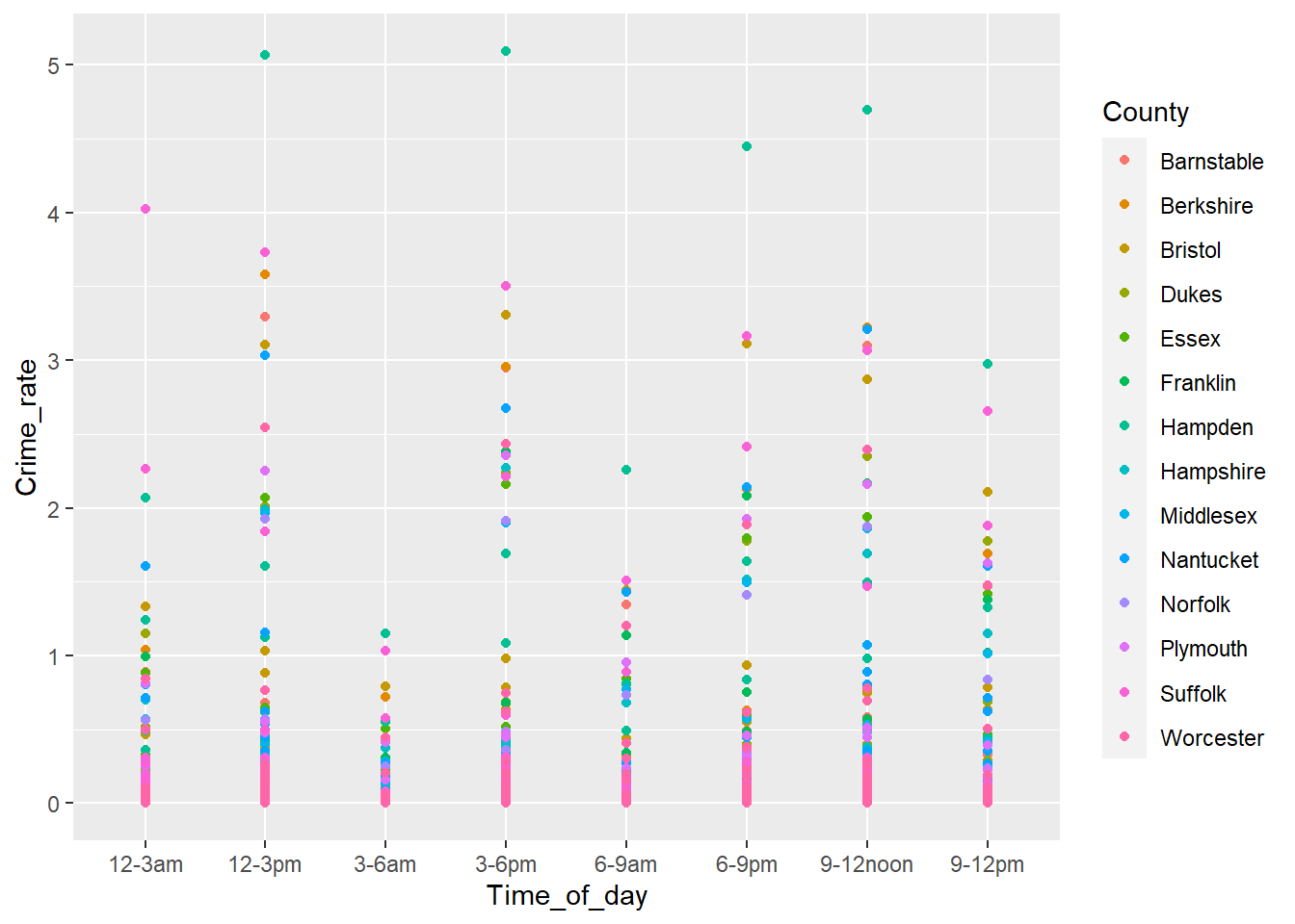
ggplot(df, aes(fill=County, y=Crime_rate, x=Time_of_day)) +
    geom_bar(position="stack", stat="identity")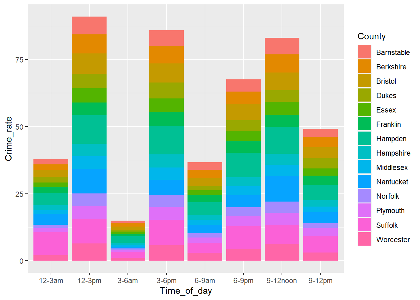
The data should be studied in depth to compare and find which time/location is safer. With the limited knowledge on R programming, I couldn’t do all the analysis that I wanted to do in the time limit. I am planning to continue working on this project as my R knowledge gets stronger.
The crime data is an interesting dataset to be studied and with the minimal resource and knowledge I have, the analysis is incomplete.