Final Project - EDA of NIFTY50 Dataset

tidyverse

final_project

Adithya Parupudi

Author

Adithya Parupudi

Published

September 3, 2022

Load Libraries

Code

library(tidyverse)
library(ggplot2)
library(ggforce)
library(forcats)
library(lubridate)
library(hrbrthemes)
library(plotly)

knitr::opts_chunk$set(echo = TRUE, warning = FALSE, message = FALSE)

Introduction

The NIFTY 50 is a benchmark Indian stock market index that represents the weighted average of 50 of the largest Indian companies listed on the National Stock Exchange. It is one of the two main stock indices used in India, the other being the BSE SENSEX. It is owned and managed by NSE Indices (previously known as India Index Services & Products Limited), which is a wholly owned subsidiary of the NSE Strategic Investment Corporation Limited. NSE Indices had a marketing and licensing agreement with Standard & Poor’s for co-branding equity indices until 2013. The Nifty 50 index was launched on 22 April 1996, and is one of the many stock indices of Nifty. The NIFTY 50 index has shaped up to be the largest single financial product in India, with an ecosystem consisting of exchange-traded funds (onshore and offshore), exchange-traded options at NSE, and futures and options abroad at the SGX. NIFTY 50 is the world’s most actively traded contract. WFE, IOM and FIA surveys endorse NSE’s leadership position.

I want to analyse the stock trends over the past decade and wanted to see if this data would give me an idea about India’s economic development. I downloaded the dataset from Kaggle and will perform an EDA of the stock prices listed from 2000 to 2021. Some answers I wanted to find out were :

D they all stocks remain the same in the NIFTY 50 index every year?
What is the best and worst stock in a year?
What is the stock performance of companies that I regularly invest in?
Which stock plummeted the most in 2008?
What are the highest and lowest stock price ever observed?

Column Descriptions

The dataset has multiple columns which tells us about the stock prices, traded volumes and son.

The column descriptions are as follows:

Date — Date of trade
symbol — Name of the company
Series — We have only one series - EQ, which stands for Equity.
Prev Close — Refers to the final price of a stock of the previous dat when the market officially closes, which is at 3:30pm IST
Open — The open is the starting period of trading on a securities exchange or organized over-the-counter market.
High — Highest price at which a stock traded during the course of the trading day.
Low — Lowest price at which a stock traded during the course of the trading day.
Last — The last price of a stock is just one price to consider when buying or selling shares. The last price is simply the most recent one
Close — The close is a reference to the end of a trading session in the financial markets when the markets close for the day.
VWAP (Volume-weighted average price)- It is the ratio of the value traded to total volume traded over a particular time horizon. It is a measure of the average price at which a stock is traded over the trading horizon
Volume — It is the amount of a security that was traded during a given period of time
Turnover -It is a measure of sellers versus buyers of a particular stock. It is calculated by dividing the daily volume of a stock by the “float” of a stock, which is the number of shares available for sale by the general trading public.
Trades- The number of shares being traded on a given day is called trading volumes
Deliverable Volume — quantity of shares which actually move from sellers to buyers
%Deliverable — shares which are actually transferred from one person’s to another’s demat account.

Read Data

There are multiple .csv files, one for each stock(around 55 files), which are located in a common folder. Using the purrr package, I am reading data from all the csv files and combining them into a single data-frame.

Code

all_stocks <- dir("_data/NIFTY_AdithyaParupudi/", full.names = TRUE) %>%  map_dfr(read_csv, )
all_stocks <- tibble(all_stocks)

The str() command gives me the column names, its datatype and first 5 observations from each column. Here we can notice that a majority of columns are numeric, one date and two character fields (stock-name). There are a total of 235192 rows, with 15 columns.

Code

str(all_stocks)

tibble [235,192 × 15] (S3: tbl_df/tbl/data.frame)
 $ Date              : Date[1:235192], format: "2007-11-27" "2007-11-28" ...
 $ Symbol            : chr [1:235192] "MUNDRAPORT" "MUNDRAPORT" "MUNDRAPORT" "MUNDRAPORT" ...
 $ Series            : chr [1:235192] "EQ" "EQ" "EQ" "EQ" ...
 $ Prev Close        : num [1:235192] 440 963 894 884 922 ...
 $ Open              : num [1:235192] 770 984 909 890 940 ...
 $ High              : num [1:235192] 1050 990 915 958 995 ...
 $ Low               : num [1:235192] 770 874 841 890 922 ...
 $ Last              : num [1:235192] 959 885 887 929 980 ...
 $ Close             : num [1:235192] 963 894 884 922 969 ...
 $ VWAP              : num [1:235192] 985 941 888 929 966 ...
 $ Volume            : num [1:235192] 27294366 4581338 5124121 4609762 2977470 ...
 $ Turnover          : num [1:235192] 2.69e+15 4.31e+14 4.55e+14 4.28e+14 2.88e+14 ...
 $ Trades            : num [1:235192] NA NA NA NA NA NA NA NA NA NA ...
 $ Deliverable Volume: num [1:235192] 9859619 1453278 1069678 1260913 816123 ...
 $ %Deliverble       : num [1:235192] 0.361 0.317 0.209 0.274 0.274 ...
 - attr(*, "spec")=
  .. cols(
  ..   Date = col_date(format = ""),
  ..   Symbol = col_character(),
  ..   Series = col_character(),
  ..   `Prev Close` = col_double(),
  ..   Open = col_double(),
  ..   High = col_double(),
  ..   Low = col_double(),
  ..   Last = col_double(),
  ..   Close = col_double(),
  ..   VWAP = col_double(),
  ..   Volume = col_double(),
  ..   Turnover = col_double(),
  ..   Trades = col_double(),
  ..   `Deliverable Volume` = col_double(),
  ..   `%Deliverble` = col_double()
  .. )
 - attr(*, "problems")=<externalptr>

Data Cleaning

Renaming column

The naming convention of last column, though intuitive, I feel would be better if I changed it to ‘PercentDeliverable’ instead of ‘%Deliverable’.

Code

all_stocksv2 <- all_stocks %>% rename(PercentDeliverable = `%Deliverble`, DeliverableVolume = `Deliverable Volume`)
colnames(all_stocksv2)

 [1] "Date"               "Symbol"             "Series"            
 [4] "Prev Close"         "Open"               "High"              
 [7] "Low"                "Last"               "Close"             
[10] "VWAP"               "Volume"             "Turnover"          
[13] "Trades"             "DeliverableVolume"  "PercentDeliverable"

Date field formatting

The date format currently available is yyyy/mm/dd. For my analysis, only the year would suffice. Hence I am creating a new column with just the ‘year’ column called ‘yy’.

Code

x<-format(as.Date(all_stocksv2$Date, format="%Y/%m/%d"))

all_stocks_yy <- all_stocksv2 %>% 
  mutate(yy=year(x)) %>%
  select(-Date)
print(all_stocks_yy)

# A tibble: 235,192 × 15
   Symbol     Series Prev C…¹  Open  High   Low  Last Close  VWAP Volume Turno…²
   <chr>      <chr>     <dbl> <dbl> <dbl> <dbl> <dbl> <dbl> <dbl>  <dbl>   <dbl>
 1 MUNDRAPORT EQ         440   770  1050   770   959   963.  985. 2.73e7 2.69e15
 2 MUNDRAPORT EQ         963.  984   990   874   885   894.  941. 4.58e6 4.31e14
 3 MUNDRAPORT EQ         894.  909   915.  841   887   884.  888. 5.12e6 4.55e14
 4 MUNDRAPORT EQ         884.  890   958   890   929   922.  929. 4.61e6 4.28e14
 5 MUNDRAPORT EQ         922.  940.  995   922   980   969.  966. 2.98e6 2.88e14
 6 MUNDRAPORT EQ         969.  985  1056   976  1049  1041. 1015. 4.85e6 4.92e14
 7 MUNDRAPORT EQ        1041. 1061  1100. 1050  1084  1082. 1083. 2.85e6 3.08e14
 8 MUNDRAPORT EQ        1082. 1089  1110. 1051  1090. 1081. 1087. 1.75e6 1.90e14
 9 MUNDRAPORT EQ        1081. 1100  1134  1078  1100  1102. 1107. 2.25e6 2.49e14
10 MUNDRAPORT EQ        1102. 1110  1110  1061. 1074. 1075. 1080. 1.01e6 1.09e14
# … with 235,182 more rows, 4 more variables: Trades <dbl>,
#   DeliverableVolume <dbl>, PercentDeliverable <dbl>, yy <dbl>, and
#   abbreviated variable names ¹`Prev Close`, ²Turnover

Summarising info and check for missing data

By running the summary command we see that Trades, Deliverable Volume and Percent_Deliverables have a lot of missing values. Since they are all numeric, I’m replacing them with 0 to avoid calculation errors.

Code

print(summarytools::dfSummary(all_stocks_yy,
                        varnumbers = FALSE,
                        plain.ascii  = FALSE, 
                        style        = "grid", 
                        graph.magnif = 0.70, 
                        valid.col    = FALSE),
      method = 'render',
      table.classes = 'table-condensed')

Data Frame Summary

all_stocks_yy

Dimensions: 235192 x 15
Duplicates: 0

Variable

Stats / Values

Freqs (% of Valid)

Graph

Missing

Symbol [character]

1. ASIANPAINT

2. BPCL

3. CIPLA

4. DRREDDY

5. GRASIM

6. HDFC

7. HDFCBANK

8. ICICIBANK

9. IOC

10. ITC

[ 55 others ]

5306	(	2.3%	)
5306	(	2.3%	)
5306	(	2.3%	)
5306	(	2.3%	)
5306	(	2.3%	)
5306	(	2.3%	)
5306	(	2.3%	)
5306	(	2.3%	)
5306	(	2.3%	)
5306	(	2.3%	)
182132	(	77.4%	)

0 (0.0%)

Series [character]

1. EQ

235192

(

100.0%

)

0 (0.0%)

Prev Close [numeric]

Mean (sd) : 1266.2 (2581.4)

min ≤ med ≤ max:

0 ≤ 566.5 ≤ 32861.9

IQR (CV) : 967.9 (2)

63729 distinct values

0 (0.0%)

Open [numeric]

Mean (sd) : 1267.8 (2585.3)

min ≤ med ≤ max:

8.5 ≤ 567 ≤ 33399.9

IQR (CV) : 968.3 (2)

44298 distinct values

0 (0.0%)

High [numeric]

Mean (sd) : 1286.6 (2619.6)

min ≤ med ≤ max:

9.8 ≤ 576.9 ≤ 33480

IQR (CV) : 983.5 (2)

49036 distinct values

0 (0.0%)

Low [numeric]

Mean (sd) : 1247.5 (2546.6)

min ≤ med ≤ max:

8.5 ≤ 556.5 ≤ 32468.1

IQR (CV) : 952.1 (2)

51335 distinct values

0 (0.0%)

Last [numeric]

Mean (sd) : 1266.4 (2581.4)

min ≤ med ≤ max:

9.1 ≤ 567 ≤ 32849

IQR (CV) : 968.5 (2)

48570 distinct values

0 (0.0%)

Close [numeric]

Mean (sd) : 1266.6 (2582.1)

min ≤ med ≤ max:

9.2 ≤ 566.7 ≤ 32861.9

IQR (CV) : 968.1 (2)

63739 distinct values

0 (0.0%)

VWAP [numeric]

Mean (sd) : 1267.1 (2582.7)

min ≤ med ≤ max:

9.2 ≤ 566.9 ≤ 32975.2

IQR (CV) : 968 (2)

138831 distinct values

0 (0.0%)

Volume [numeric]

Mean (sd) : 3045903 (7333981)

min ≤ med ≤ max:

3 ≤ 1010939 ≤ 481058927

IQR (CV) : 2800842 (2.4)

220434 distinct values

0 (0.0%)

Turnover [numeric]

Mean (sd) : 1.610138e+14 (3.298085e+14)

min ≤ med ≤ max:

10470000 ≤ 6.832603e+13 ≤ 3.564334e+16

IQR (CV) : 1.702553e+14 (2)

235184 distinct values

0 (0.0%)

Trades [numeric]

Mean (sd) : 61964.3 (68664.6)

min ≤ med ≤ max:

11 ≤ 44068 ≤ 1643015

IQR (CV) : 57101.5 (1.1)

79112 distinct values

114848 (48.8%)

DeliverableVolume [numeric]

Mean (sd) : 1315098 (2831670)

min ≤ med ≤ max:

5 ≤ 501756 ≤ 232530747

IQR (CV) : 1326850 (2.2)

199963 distinct values

16077 (6.8%)

PercentDeliverable [numeric]

Mean (sd) : 0.5 (0.2)

min ≤ med ≤ max:

0 ≤ 0.5 ≤ 1

IQR (CV) : 0.3 (0.4)

9456 distinct values

16077 (6.8%)

yy [numeric]

Mean (sd) : 2010.9 (5.9)

min ≤ med ≤ max:

2000 ≤ 2011 ≤ 2021

IQR (CV) : 10 (0)

22 distinct values

0 (0.0%)

Generated by summarytools 1.0.1 (R version 4.2.1)
2022-12-23

Replacing NA’s with 0’s

I’ve observed there are NA values in 3 columns. To avoid calculation/code errors, I decided to replace all NA’s with 0. Also, replacing by zero doesn’t have any impact on the observations because, the stock was not traded when it was first listen in the NIFTY index.

By using replace_na() function, I’ve picked 3 columns as a result of the above observations made from the summary table.

Code

# all_stocks_yy[is.na(all_stocks_yy)] <- 0
# sum(is.na(all_stocks_yy$Trades))
# 
# 
# all_stocks_yy %>% mutate(
#     across(everything(), ~replace_na(., 0))
#   )

all_stocks_yy <- all_stocks_yy %>% replace_na(list(PercentDeliverable = 0, DeliverableVolume = 0, Trades=0))

Observations

Distinct stocks

NIFTY50 is supposed to be the top 50 stocks of the financial year(there must be 50 distinct stocks in the data set). This data from 2000 to 2021 is not consistent, i.e., there are 65 distinct entries found. Which suggests that some stocks under-performed and got replaced with new ones over time. Hence the aggregate of all stocks combined became 65

Code

all_stocks_yy %>% select(1) %>% distinct()

# A tibble: 65 × 1
   Symbol    
   <chr>     
 1 MUNDRAPORT
 2 ADANIPORTS
 3 ASIANPAINT
 4 UTIBANK   
 5 AXISBANK  
 6 BAJAJ-AUTO
 7 BAJAJFINSV
 8 BAJAUTOFIN
 9 BAJFINANCE
10 BHARTI    
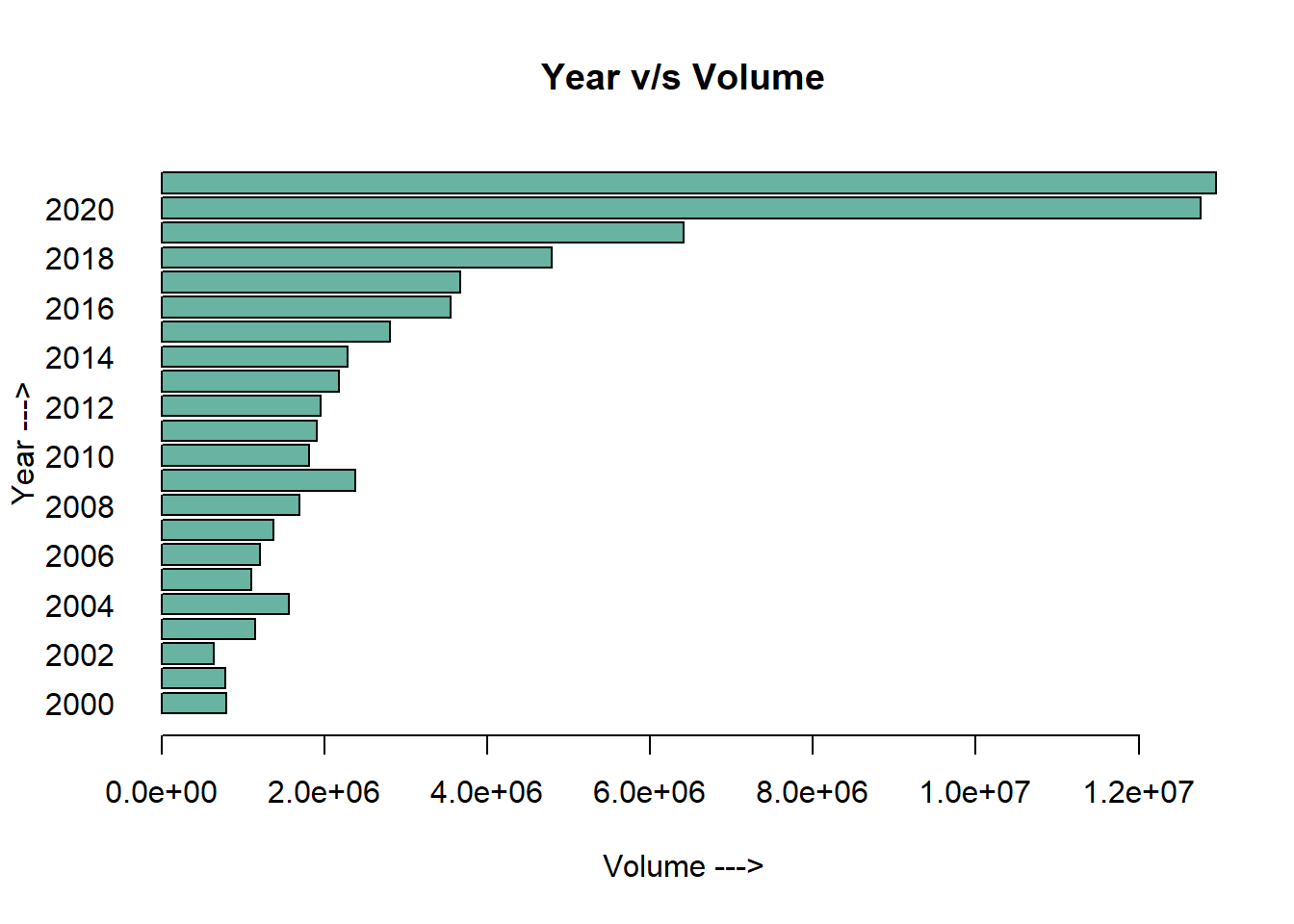
# … with 55 more rows

Year vs Volume of stock traded

We can infer from the mean of Volume column, the number of stocks sold each year kept increasing.

This can hint an increase in demat accounts and number of active trading as well.
New stocks must have entered the NIFTY50 index, and started performing well over the years
Special attention can be paid to volumes of stock sold between 2018 - 2021. There is a sharp increase in the volume of shares traded. Due to the COVID-19 pandemic, many stocks fell which encouraged more people than ever to open a demat account and start investing( I opened mine during this time!!!)

Code

barplot<- all_stocks_yy %>% 
  group_by(yy) %>% 
  select(`Volume`) %>% 
  summarise_all(mean, na.rm=TRUE)

barplot(height=barplot$Volume, names=barplot$yy, 
        col="#69b3a2",
        horiz=T, las=1,
        xlab='Volume --->',
        ylab='Year --->',
        main='Year v/s Volume',
        )

Checking stock’s consistency in NIFTY50 index

By running the below code, I am checking whether a stock has maintained its consistency in the top 50 stocks. Looks like the stocks kept changing each year, and some stocks were not present in the list at all! The stocks not present in that year can be identified with 0 ( a metric for the sum of all shares sold in a year ). That is, if no shares are sold, then the stock wouldn’t make the list.

Some observations that can be made here are:

Stocks like ADANIPORTS, NESTLEIND, NTPC, SSLT didn’t enter the stock market from 2000. Their companies began appearing further down the line, such as from 2010
Some companies, though made it to the NIFTY 50 list, have dropped out over the years due to a massive dip in stock price due to various factors. Some such examples would be KOTAKMAH, INFOSYSTCH, TELCO, TISCO have experienced huge losses which can be explained change in their leadership, an acquisition gone wrong, or someone filed a case in the court.

From my understanding so far, a stock price dips heavily due to change in public sentiment, as a direct impact of news channels.

Code

all_stocks_yy %>% 
  pivot_wider(names_from=`yy`, values_from = `Volume`) %>% 
  group_by(Symbol) %>% select(Trades, 14:35) %>% 
  summarise_all(sum, na.rm=TRUE) %>% 
  relocate(`2000`:`2006`, .before = `2007`)

# A tibble: 65 × 24
   Symbol  Trades `2000` `2001` `2002` `2003` `2004` `2005` `2006` `2007` `2008`
   <chr>    <dbl>  <dbl>  <dbl>  <dbl>  <dbl>  <dbl>  <dbl>  <dbl>  <dbl>  <dbl>
 1 ADANIP… 1.08e8 0      0      0      0      0      0      0      0      0     
 2 ASIANP… 1.02e8 3.55e6 4.45e6 3.99e6 6.10e6 7.93e6 8.78e6 7.61e6 9.96e6 8.48e6
 3 AXISBA… 2.96e8 0      0      0      0      0      0      0      6.71e7 5.79e8
 4 BAJAJ-… 6.75e7 0      0      0      0      0      0      0      0      3.07e7
 5 BAJAJF… 5.13e7 0      0      0      0      0      0      0      0      5.30e7
 6 BAJAUT… 0      6.06e5 2.69e5 1.06e6 2.68e6 3.60e6 4.07e6 2.32e6 3.96e6 6.42e6
 7 BAJFIN… 1.39e8 0      0      0      0      0      0      0      0      0     
 8 BHARTI  0      0      0      9.55e7 3.23e8 8.80e8 4.36e8 8.82e7 0      0     
 9 BHARTI… 2.09e8 0      0      0      0      0      0      1.21e8 4.55e8 9.59e8
10 BPCL    1.37e8 2.12e7 5.39e7 3.90e8 3.51e8 2.27e8 1.12e8 1.10e8 1.27e8 1.66e8
# … with 55 more rows, and 13 more variables: `2009` <dbl>, `2010` <dbl>,
#   `2011` <dbl>, `2012` <dbl>, `2013` <dbl>, `2014` <dbl>, `2015` <dbl>,
#   `2016` <dbl>, `2017` <dbl>, `2018` <dbl>, `2019` <dbl>, `2020` <dbl>,
#   `2021` <dbl>

Stocks which didn’t enter stock market for 10 yrs

There are 6 stocks which did not enter the stock market - ADANIPORTS, HEROMOTOCO, INFY,SSLT,UPL, VEDL. They were not publicly listed in to be traded, as the company was still small in size. A company enters stock market once it has captured enough market in an area, and wants to expand its operations and brand to a larger scale. The companies then offer IPO, where the shares are made available to common people to invest. Using this additional income, the companies expand their scale of operations to PAN_India!

Code

all_stocks_yy %>% 
  pivot_wider(names_from=`yy`, values_from = `Volume`) %>% 
  group_by(Symbol) %>% select(Trades, 14:35) %>% 
  summarise_all(sum, na.rm=TRUE) %>% 
  relocate(`2000`:`2006`, .before = `2007`) %>% 
  select(`Symbol`, `2000`:`2010`) %>% 
  filter(across(`2000`:`2010`, ~ . ==0)) %>% 
  select(Symbol)

# A tibble: 6 × 1
  Symbol    
  <chr>     
1 ADANIPORTS
2 HEROMOTOCO
3 INFY      
4 SSLT      
5 UPL       
6 VEDL

Best and Worst Performing Stock of 2000

ZEETELE - Best performing stock in 2000, AJAUTOFIN - Worst performing stock 2000. They are calculated based on their cumulative volumes of all the years respectively

Code

# best performing stock
all_stocks_yy %>% 
  group_by(yy, Symbol) %>% 
  select(`Volume`) %>% 
  summarise_all(sum, na.rm=TRUE) %>% 
  arrange(desc(Volume)) %>% 
  slice(1)

# A tibble: 22 × 3
# Groups:   yy [22]
      yy Symbol        Volume
   <dbl> <chr>          <dbl>
 1  2000 ZEETELE   2124967599
 2  2001 ZEETELE   2136706114
 3  2002 ZEETELE   1402554565
 4  2003 TISCO     1674239842
 5  2004 TISCO     2026827972
 6  2005 RELIANCE  1423512801
 7  2006 ITC       1495441954
 8  2007 POWERGRID 1985771033
 9  2008 NTPC      1988073378
10  2009 TATASTEEL 2577318306
# … with 12 more rows

Code

# worst performing stock
all_stocks_yy %>% 
  group_by(yy, Symbol) %>% 
  select(`Volume`) %>% 
  summarise_all(sum, na.rm=TRUE) %>% 
  arrange(Volume) %>% 
  slice(1)

# A tibble: 22 × 3
# Groups:   yy [22]
      yy Symbol      Volume
   <dbl> <chr>        <dbl>
 1  2000 BAJAUTOFIN  606464
 2  2001 BAJAUTOFIN  269290
 3  2002 BAJAUTOFIN 1059613
 4  2003 BRITANNIA  2557859
 5  2004 BRITANNIA  3351970
 6  2005 BRITANNIA  1998097
 7  2006 BRITANNIA  1503856
 8  2007 BRITANNIA  2629574
 9  2008 BRITANNIA  1561330
10  2009 BRITANNIA  1754997
# … with 12 more rows

Plotting the above results

I have created a scatterplot for the best and the worst stock as shown below. It was surprising to see such a sharp decline in traded volumes for ZEETELE just the corresponding year. And the worst performing stock of 2000 gradually gained traction and crossed the aforementioned stock in the year 2006.

The dip in stock volume is observed for BAJAUTOFIN due to the stock market crash, but still continues to maintain its position in the NIFTY index. Looks like ZEETELE got kicked of the NIFTY index at the beginning of 2007

This link describes about the US stock market crash after the attack on World Trade Center on Sept 11, 2001. The corresponding events led to stock crash world wide, thus effecting Indian markets as well. ZEETELE is one of those stock which got highly effected. In the following years, many stocks failed to make a come back and also got replaced by other stocks in the NIFTY index.

Red line - BAJAUTOFIN , Blue Line - ZEETELE

Code

p<-all_stocks_yy %>% 
  select(Symbol, yy, `Prev Close`) %>% 
  filter(Symbol == "ZEETELE" | Symbol == "BAJAUTOFIN") %>% 
  group_by(yy, Symbol) %>% 
  summarize_all(mean, na.rm = TRUE) %>% 
  pivot_wider(names_from = Symbol, values_from = `Prev Close`) %>% 
  ggplot()+
  geom_line(aes(x=yy, y=BAJAUTOFIN), color='red') + 
  geom_point(aes(x=yy, y=BAJAUTOFIN),size=1.5, color='red') + 
  geom_line(aes(x=yy, y=ZEETELE), color='blue') + 
  geom_point(aes(x=yy, y=ZEETELE),size=1.5, color="blue") +   
  labs(title='ZEETELE, BAJAUTOFIN - Stock performance', x="Year", y="Previous Close") + theme_bw() 

ggplotly(p)

Best and Worst stock of 2021 by Volume

Best performing stock was TATAMOTORS, and the worst performing stock was SHREECEM

Code

# best performing stock of 2021
all_stocks_yy %>% 
  group_by(yy, Symbol) %>% 
  select(`Volume`) %>% 
  summarise_all(sum, na.rm=TRUE) %>% 
  arrange(desc(Volume)) %>% 
  filter(yy==2021) %>% 
  head()

# A tibble: 6 × 3
# Groups:   yy [1]
     yy Symbol         Volume
  <dbl> <chr>           <dbl>
1  2021 TATAMOTORS 7724352104
2  2021 SBIN       4088703389
3  2021 ITC        2982397228
4  2021 ONGC       2501344432
5  2021 NTPC       2132902536
6  2021 IOC        2072409999

Code

# worst performing stock of 2021
all_stocks_yy %>% 
  group_by(yy, Symbol) %>% 
  select(`Volume`) %>% 
  summarise_all(sum, na.rm=TRUE) %>% 
  arrange(Volume) %>% 
  filter(yy==2021) %>% 
  head()

# A tibble: 6 × 3
# Groups:   yy [1]
     yy Symbol       Volume
  <dbl> <chr>         <dbl>
1  2021 SHREECEM    5311556
2  2021 NESTLEIND   9157164
3  2021 BAJAJFINSV 48075888
4  2021 BRITANNIA  54033577
5  2021 ULTRACEMCO 56268478
6  2021 BAJAJ-AUTO 68826756

Plotting the above results

Over the years, SHREECEM have observed a steady growth. Its a cement manufacturing company from Rajasthan, who played a valuable role in India’s development.

Code

stocks_2021<-all_stocks_yy %>% 
  select(Symbol, yy, `Prev Close`) %>% 
  filter(Symbol == "TATAMOTORS" | Symbol == "SHREECEM") %>% 
  group_by(yy, Symbol) %>% 
  summarize_all(mean, na.rm = TRUE) %>% 
  pivot_wider(names_from = Symbol, values_from = `Prev Close`) %>% 
  ggplot()+
  geom_line(aes(x=yy, y=SHREECEM), color='red') + 
  geom_point(aes(x=yy, y=SHREECEM),size=1.5, color='red') + 
  geom_line(aes(x=yy, y=TATAMOTORS), color='blue') + 
  geom_point(aes(x=yy, y=TATAMOTORS),size=1.5, color="blue") +   
  labs(title='TATAMOTORS, SHREECEM - Stock performance', x="Year", y="Previous Close") + theme_bw() 

ggplotly(stocks_2021)

Which stock plummeted the most in 2008?

The answer to that question is SESAGOA - an Iron Ore company in Goa

Code

stocks_2008 <- all_stocks_yy %>% filter(`yy` == 2008) %>% 
  select(yy, Symbol, `Prev Close`) %>% 
  group_by(Symbol,yy) %>% 
  summarise_all(median, na.rm=TRUE) %>% 
  ungroup() %>% 
  arrange(desc(`Prev Close`)) %>% 
  head()

bar_2008<- stocks_2008 %>% ggplot(aes(x=`Prev Close`, y=Symbol, color=yy)) + 
  geom_bar(stat="identity", fill="#f68060", alpha=.6, width=.4) +
    theme_bw()

ggplotly(bar_2008)

Stock performance between 2018 to 2021

I’ve picked a few stocks whose brands I am most familiar with and use their services in daily life. It was interesting to see that Britannia and HDFC stocks fell by a large number and quickly recovered in 2021. Their brand image is really good in the Indian market and they are immune to market volatility. These are some of the best long term investment options.

Code

stock_perf <- all_stocks_yy %>% 
  filter(`yy` == 2018 | `yy` == 2019 | `yy` == 2020 |`yy` == 2021) %>% 
   filter(Symbol == 'ADANIPORTS' |
Symbol == 'ASIANPAINT' | Symbol == 'BRITANNIA' | Symbol == 'INFY' | Symbol == 'CIPLA' | Symbol == 'HDFCBANK' | Symbol == 'RELIANCE' | Symbol == 'TCS' |Symbol == 'TECHM') %>% 
   select(yy,Symbol, `Prev Close`) %>% 
   group_by(Symbol,yy) %>% 
   arrange(`Prev Close`) %>% 
   slice(1) 

 
stock_perf%>% ggplot( aes(x=yy,y=`Prev Close`, label = yy)) +
    geom_line( color="grey") +
    geom_point(color="blue", size=2) +
  facet_wrap(~Symbol,nrow =4) +
  labs(x='year', y='Prev Close')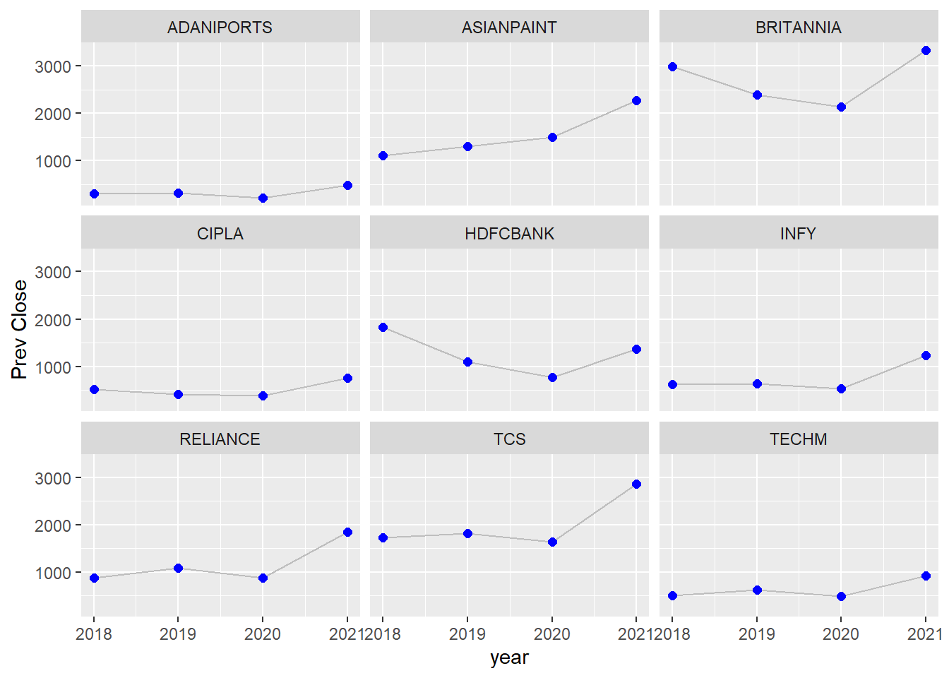

Code

    ggtitle("Stock performance during COVID-19") + theme_dark()

NULL

Highest and Lowest stock prices observed in dataset

Calculating this based on Prev Close column, which tells the last traded price of the stock.

Highest price is observed for EICHERMOT aka Eicher Motors Ltd in 2017, traded at 32,861.95 rupees per share. It is an Indian MNC which manufactures motorcycles and commercial vehicles, headquartered in New Delhi.

Lowest prices don’t really count as per the code because the stock price is close to 0 when it enters the stock market.

Code

all_stocks_yy %>% 
  select(Symbol, `Prev Close`, yy) %>% 
  arrange(desc(`Prev Close`)) %>% 
  head()

# A tibble: 6 × 3
  Symbol    `Prev Close`    yy
  <chr>            <dbl> <dbl>
1 EICHERMOT       32862.  2017
2 EICHERMOT       32766.  2017
3 EICHERMOT       32662.  2017
4 EICHERMOT       32618.  2017
5 EICHERMOT       32499.  2017
6 EICHERMOT       32444.  2017

Code

all_stocks_yy %>% 
  select(Symbol, `Prev Close`, yy) %>% 
  arrange(`Prev Close`) %>% 
  head()

# A tibble: 6 × 3
  Symbol     `Prev Close`    yy
  <chr>             <dbl> <dbl>
1 BHARTI             0     2002
2 LT                 2     2004
3 INDUSINDBK         9.15  2001
4 INDUSINDBK         9.4   2001
5 INDUSINDBK         9.5   2001
6 INDUSINDBK         9.6   2001

Which stock consistently maintained its position for the longest time?

Below are the list of 23 stocks which are consistently a part of NIFTY. Just like all the other stocks, they also experienced heavy price drops, but also gained the market share just as fast. These are the best performing stocks of the Indian market and we can safely invest in them for the long run.

Code

all_stocks_yy %>% 
  pivot_wider(names_from=`yy`, values_from = `Volume`) %>% 
  group_by(Symbol) %>% select(Trades, 14:35) %>% 
  summarise_all(sum, na.rm=TRUE) %>% 
  relocate(`2000`:`2006`, .before = `2007`) %>% 
  select(`Symbol`, `2000`:`2021`) %>% 
  filter(across(`2000`:`2021`, ~ . !=0)) %>% 
  select(Symbol)

# A tibble: 23 × 1
   Symbol    
   <chr>     
 1 ASIANPAINT
 2 BPCL      
 3 BRITANNIA 
 4 CIPLA     
 5 DRREDDY   
 6 EICHERMOT 
 7 GAIL      
 8 GRASIM    
 9 HCLTECH   
10 HDFC      
# … with 13 more rows

Reflection

This project has been a great learning experience for me. It was interesting to see how many insights can be derived from a single data set. I felt that I barely scratched the surface of this goldmine dataset. I used to follow stock market trends for a while during the covid lockdown, which made me interested to try this do an EDA of this data-set. My current regret is, there are lot of amazing insights and visualizations that I could do, but I didn’t know how to manipulate multiple variables to make it happen.

I faced challenges with almost every aspect of this project. I’ve been going back to my notes, stack overflow and a bunch of youtube videos to get clarity. I made use of really good websites and bookmarked some of the solutions for future reference. There is a lot of power in R and it made me realize I could really do a lot more with it.

I’ve made use of other packages apart from the standard ones taught in the class, and tried resolving multiple errors by fine-tuning the functions. There is still a lot more to learn, and I will continue learning to be better at visualization.

Conclusion

I got some clarity on the highs and lows of the stock market. A stock doesn’t appear to be consistent in the NIFTY index and new ones get added or replaced each consecutive year. Sometimes the stocks start at a very high price, but plummets almost immediately the next year,which makes it very dangerous to have had shares in that stock(,i.e., ZEETELE). Some stocks stood the test of time and their brand image grew bigger. Not all stocks started out at year 2000, while some of them entered almost 10 years later and continued to be in the NIFTY index. While some stocks changed considerably due to world events such as terrorist attacks on WTC, Covid 19, Wall Street crash etc, not all stocks managed to recover.

A stock’ss performance is directly proportional to its public image. The stock price immediately drops if the company’s image is tarnished. The number of people who started investing grew each year, and the highest jump in the traded volumes can be observed between 2018 to 2021, a direct consequence of COVID-19 pandemic. Since people were restricted at home, there was a lot of surplus money sitting idly in their bank accounts. Therefore they invested in the stock markets which were crashing due to the declining businesses. All the NIFTY stocks will rise each time they fall, is what I’ve observed, but stocks from the manufacturing industry will only experience temporary dips in price.

As India is a developing country, there is a continuous involvement of the manufacturing industry. So even if there is a plateau in price, the price and public sentiment will eventually rise.

Bibliography

Dataset from kaggle - https://www.kaggle.com/datasets/rohanrao/nifty50-stock-market-data

Definitions - https://en.wikipedia.org/wiki/NIFTY_50