#install.packages("treemap")
#install.packages("treemapify")
#install.packages("usmap")
#install.packages("ggalluvial")
#install.packages("reshape")
library(reshape)
library(usmap)
library(tidyverse)
library(ggplot2)
library(readr)
library(summarytools)
library(plotly)
library(stringr)
library(ggalluvial)
library(readxl)
library(treemap)
library(treemapify)

knitr::opts_chunk$set(echo = TRUE, warning=FALSE, message=FALSE)Cancer Incidence and Mortality Analysis across States and Age Groups
Final Project
Animesh Sengupta
Census Data
Cancer USPS Data
Exploratory analysis of Cancer incidence and mortality rate against the US population data between the years 2000-2019, grouped by State and Age Groups
Project Overview
This current project is the exploratory analysis for DACSS 601 Fundamentals of Data Science - Final Project of US Cancer Data grouped by Area, Age groups and Race against the Census population grouped by the same parameters across the year 2000 to 2020.
This project contains the following sections:
- Introduction & Motivation
- US Cancer Statistics grouped by Area - Tidying and Sanitation
- US Census Data grouped by Area - Tidying and Sanitation
- US Census Data grouped by Area - Analysis
- US Cancer vs Census Data grouped by Area Parameter - Join and Analysis
- US Census Data grouped by Age groups - Tidying and Sanitation
- US Cancer Statistics grouped by Age groups - Tidying and Sanitation
- US Cancer Statistics grouped by Age groups - Analysis
- US Cancer vs Census Data grouped by Age Parameter - Join and Analysis
- Conclusion
- References
Introduction and Motivation
In the past few decades, our species have made significant strides in improving the medical facilities and technologies thus significantly improving our lifespans and quality of life. Even after such amazing technological feats and centuries of study of the human body, Cancer proves to be a thorn in our path. Cancer is one of the biggest chronic illnesses plaguing multiple people across the planet throughout decades. Since then, the solution to evade and treat Cancer is amongst the hottest topic in the scientific field and the research around its inception, is even more critical.
In the ever changing world dynamics with overpopulation and pollution plaguing our societies, cancer has not only increased but has become prevalent. This small study aims to find questions regarding the incidence and mortality statistics across the US States and population. More Importantly this study aims to find how prevalent different types of Cancer are in the state. This study will also outline the spread of cancer among different age groups of US population as well. So in essance, in this study we are determined to ask two major questions:
- How is cancer incidence and mortality cases spread across the states over the last 2 decades?
- How is Cancer incidence spread across different age groups in the US population?
To understand the following two questions, we are using two US government published datasets. They are as follow:
- US cancer statistics dataset: Maintained and procured by the CDC WONDER org.[1]
- US Census Bureau Population dataset.[2]
##US Cancer Statistics grouped by Area - Tidying and sanitation.
USCS_Area <- read_csv("../posts/_data/Animesh_data/USCS_Area1.csv")
USCS_Area<-USCS_Area%>%select(AREA,YEAR,SITE,EVENT_TYPE,COUNT)%>%
  filter(YEAR!='1999')%>%
  filter(COUNT!="~" & COUNT!="+" & COUNT!="." & COUNT!="-")%>%
  mutate(YEAR=as.double(YEAR),
         COUNT=as.double(COUNT))%>%
  drop_na(YEAR,AREA)%>%
  unique()
view(dfSummary(USCS_Area))
head(USCS_Area,5)
# A tibble: 5 × 5
AREA YEAR SITE EVENT_TYPE COUNT
<chr> <dbl> <chr> <chr> <dbl>
1 Alabama 2000 All Cancer Sites Combined Incidence 9475
2 Alabama 2000 All Cancer Sites Combined Mortality 4425
3 Alabama 2001 All Cancer Sites Combined Incidence 9971
4 Alabama 2001 All Cancer Sites Combined Mortality 4550
5 Alabama 2002 All Cancer Sites Combined Incidence 10152Our first step would be to read the raw data provided by the US cancer statistics dataset and tidying it according to our needs. This dataset has the following dimensions 332532, 5. The USCS raw data had a lot of statistical features, which wont be required for the study and thus were trimmed. The selected features of the dataset are AREA, YEAR, SITE, EVENT_TYPE, COUNT.
After careful consideration from viewing the dataframe summary of the data, the following tidying and sanitation actions were performed: 1. Only the relevant features were selected and statistical features were trimmed from the dataset. 2. The Year 1999 data was filtered out, because we are only concerened about the 2000-2019 3. The type of feature Year and Count were converted from char to double 4. duplicates rows were removed 5. Rows with NA in year and area were also dropped to maintain consistency.
From the dfsummary, we can check that the year are of proper type and runs from 2000-2019. All the other features types are as expected and there are no duplicate values either.
US Census Data grouped by Area - Tidying and Sanitation
One of the most challenging task was to extract the right dataset/table from the US Census datasets. To analyse the cancer trend among US population, we need the state wise US population statistics.
We extracted the state wise population statistics for two decades i.e 2000-2010 and 2011-2020. The following code snippets extracts the data
area_2000_Data<-read_excel("../posts/_data/Animesh_data/2000s_state_data.xls",
    skip = 4, n_max = 60,col_names=c("Area","2009","2008","2007","2006","2005","2004","2003","2002","2001","2000","April_2000_estimate","April_2000_census"))
area_2000_Data<-area_2000_Data%>%select(-one_of(c("April_2000_census","April_2000_estimate")))%>%
  pivot_longer(
    cols=starts_with("20"),
    names_to = "Year",
    names_transform = list(Year = as.double),
    values_to= "Population_count"
  )
The following dataset had year as features. The following tidying actions were perfomed
- As a rule of thumb , all the population estimates figure for the years were taken on July 1. In that extent, the population estimate of 2010 was also chosen when presented with both April and July,2010 data. The rest of the data was skimmed
- The Year columns were pivoted longer and converted into row data.
- Appropriate numerical columns were converted from char to double
The similar approach was also taken for the 2010 decade dataset. Similar features were present in this dataset too and thus a similar tidying approach were taken to tidy this too. Refer to the code below
area_2010_Data<-read_excel("../posts/_data/Animesh_data/2010s_state_data.xlsx",
    skip = 4, n_max = 60,col_names=c("Area","April_2010_estimate","April_2010_census","2010","2011","2012","2013","2014","2015","2016","2017","2018","2019","April_2020_estimate","2020"))
area_2010_Data<-area_2010_Data%>%select(-one_of(c("April_2010_census","April_2010_estimate","April_2020_estimate")))%>%
  pivot_longer(
    cols=starts_with("20"),
    names_to = "Year",
    names_transform = list(Year = as.double),
    values_to= "Population_count"
  )
Since most of the features were similar between the two dataset, similar tidying principles were applied. Our aim is to make both the dataframe homogenous for them to stack together appropriately. Our ulterior motive is to get a singular dataframe with Area statistics for both the decades.
Once both the data was extracted , we stacked them together. In addition to this, we also needed the State codes and abbreviation for our visualization purposes. In the code snippet below, we also extract a State to abbreviation mapping and join it to our Census dataset.
area_data<-bind_rows(area_2000_Data,area_2010_Data)
area_data$Area<-str_remove(area_data$Area,"[[:punct:]]")
area_code <- read_csv("../posts/_data/Animesh_data/state_code.csv")
area_data_code<-merge(area_data,area_code,by.x=c("Area"),by.y=c("State"))
head(area_data_code,10)
Area Year Population_count Abbreviation
1 Alabama 2007 4637904 AL
2 Alabama 2006 4597688 AL
3 Alabama 2005 4545049 AL
4 Alabama 2008 4677464 AL
5 Alabama 2003 4490591 AL
6 Alabama 2002 4472420 AL
7 Alabama 2001 4464034 AL
8 Alabama 2004 4512190 AL
9 Alabama 2010 4785514 AL
10 Alabama 2011 4799642 ALNow we have a dataframe containing the population change across different states over 2 decades. The dimensions of the dataset are 1071, 4. While the features for this dataset are Area, Year, Population_count, Abbreviation.
US Census Data grouped by Area - Analysis
One of the most important aspect of population is to find out the rate of change of population across different states. This trend can prove to be a very important indicator in access to healthcare and important medicare resources across the states. Usually a buregoning population will have stressed resources and thus higher percentage of people with poor access to the healthcare Infra.
jarea_gg1<-ggplot(area_data_code,aes(x=Year,y=Population_count,color=Area))+
  geom_line()+
  ylab("Population Count")+
  ggtitle("Change in population from 2000-2020 in US States")
ggplotly(jarea_gg1)
As per the above visualization, The state of califoria has the highest population across the two decades. While the state of Texas has the steepest slope , hence have the highest rate of growth.
jarea_gg2<-ggplot(area_data_code%>%filter(Year=="2020"),aes(area=Population_count,fill=Abbreviation, label=Abbreviation))+
  geom_treemap()+
  geom_treemap_text(colour = "white",
                    place = "centre",
                    size = 10) +
  theme(legend.position = "none")+
  ggtitle("State-wise Population Density for the Year 2020")
jarea_gg2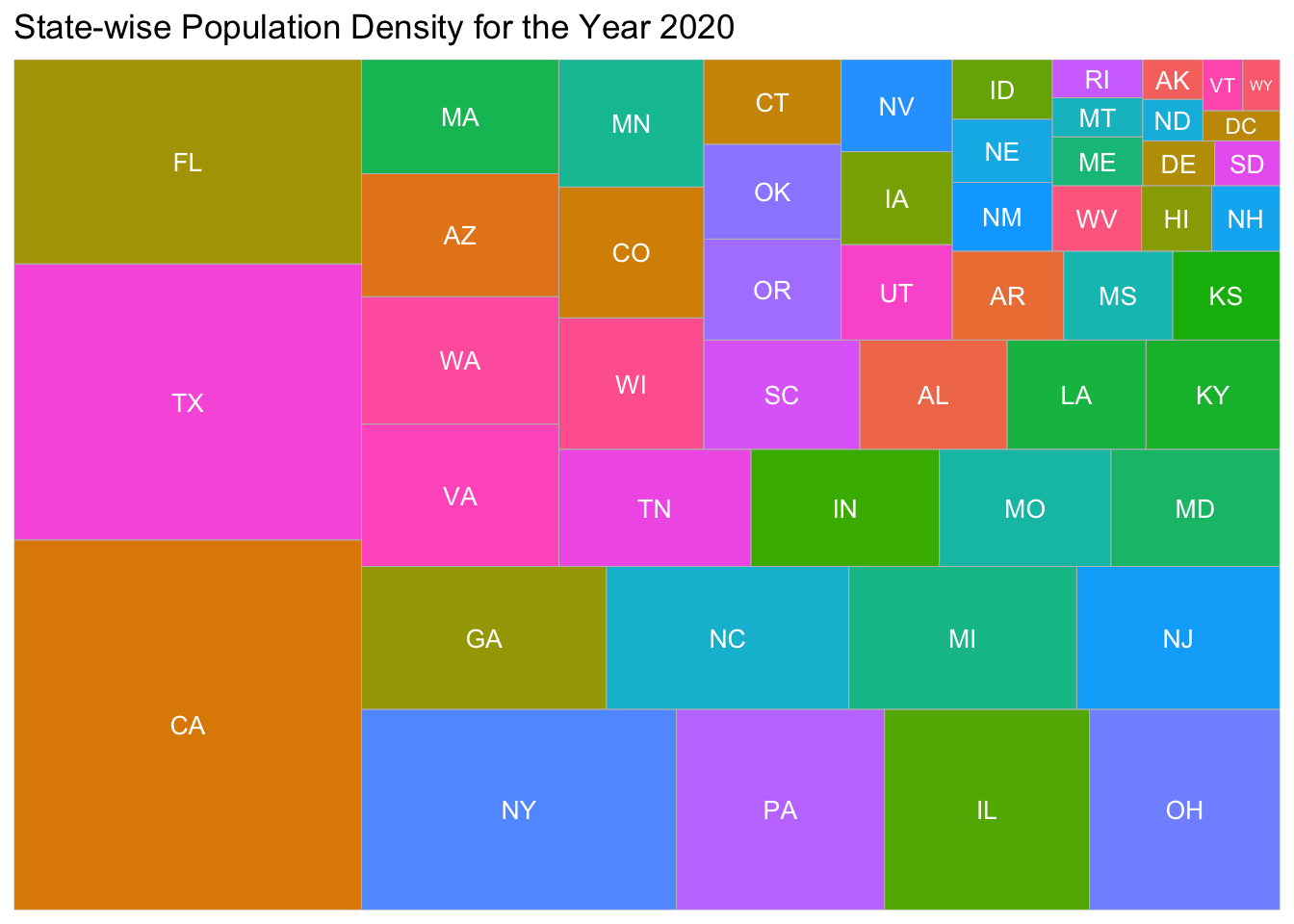
We are also concerned about the population densty among the states. The above treemap paints a very good picture on where the population is scattered at. From the visualization we can observe that the state of California and Texas are the most populous state while Wyoming is less populated.
We chose the Treemap visualization to effectively show the population density amongst the states without cluttering the graphs. A treemap was the best visual tool to show the population size compared to different states.
US Cancer vs Census Data grouped by Area Parameter - Join and Analysis
One of the important features of the USCS Cancer data is the count of cancer cases for a particular area. If we also have the population data for that area and year, we can identify the percentage of population affected by cancer.
To achieve this, we perform a inner join between the Cancer Dataset and US census data over the Area and Year features.
Area_joined<-merge(USCS_Area,area_data_code,by.x=c("AREA","YEAR"), by.y=c("Area","Year"))

view(dfSummary(Area_joined))

Area_wise_cancer<-Area_joined%>%
  filter(SITE=="All Cancer Sites Combined")%>%
  filter(YEAR=="2000"|YEAR=="2010"|YEAR==
           "2019")%>%
  group_by(AREA,YEAR,SITE,Abbreviation,Population_count,EVENT_TYPE)%>%
  summarize(Nct=sum(COUNT))%>%
  mutate("Count_percent"=Nct/Population_count*100)%>%
  dplyr::rename(state=AREA)%>%
  ungroup()

head(Area_wise_cancer,20)
# A tibble: 20 × 8
state YEAR SITE Abbre…¹ Popul…² EVENT…³ Nct Count…⁴
<chr> <dbl> <chr> <chr> <dbl> <chr> <dbl> <dbl>
1 Alabama 2000 All Cancer Sites Combi… AL 4451849 Incide… 79242 1.78
2 Alabama 2000 All Cancer Sites Combi… AL 4451849 Mortal… 39188 0.880
3 Alabama 2010 All Cancer Sites Combi… AL 4785514 Incide… 101355 2.12
4 Alabama 2010 All Cancer Sites Combi… AL 4785514 Mortal… 40832 0.853
5 Alabama 2019 All Cancer Sites Combi… AL 4907965 Incide… 110363 2.25
6 Alabama 2019 All Cancer Sites Combi… AL 4907965 Mortal… 41164 0.839
7 Alaska 2000 All Cancer Sites Combi… AK 627499 Incide… 8247 1.31
8 Alaska 2000 All Cancer Sites Combi… AK 627499 Mortal… 2770 0.441
9 Alaska 2010 All Cancer Sites Combi… AK 713982 Incide… 11472 1.61
10 Alaska 2010 All Cancer Sites Combi… AK 713982 Mortal… 3508 0.491
11 Alaska 2019 All Cancer Sites Combi… AK 733603 Incide… 12740 1.74
12 Alaska 2019 All Cancer Sites Combi… AK 733603 Mortal… 4116 0.561
13 Arizona 2000 All Cancer Sites Combi… AZ 5166697 Incide… 92508 1.79
14 Arizona 2000 All Cancer Sites Combi… AZ 5166697 Mortal… 37896 0.733
15 Arizona 2010 All Cancer Sites Combi… AZ 6407342 Incide… 121592 1.90
16 Arizona 2010 All Cancer Sites Combi… AZ 6407342 Mortal… 45020 0.703
17 Arizona 2019 All Cancer Sites Combi… AZ 7291843 Incide… 141332 1.94
18 Arizona 2019 All Cancer Sites Combi… AZ 7291843 Mortal… 53432 0.733
19 Arkansas 2000 All Cancer Sites Combi… AR 2678288 Incide… 50996 1.90
20 Arkansas 2000 All Cancer Sites Combi… AR 2678288 Mortal… 24314 0.908
# … with abbreviated variable names ¹Abbreviation, ²Population_count,
# ³EVENT_TYPE, ⁴Count_percentTo further fit the data to the require visualizations, we chose a subset of datasets. In our analysis, we can look into the change in % population during the turn of century. So for the year 2000,2010 and 2019, we plotted the %Count of the population affected by Cancer and died by cancer. To acheive this we did the following actions: 1. Removed the “All cancer sites combined” parameter from Cancer Sites. 2. Chose 2000,2010 and 2019 as subset years 3. grouped according to Area year and site while summing the count. 4. Converted the feature name of Area to state for USmap package.
area_gg1<-plot_usmap(data=Area_wise_cancer%>%filter(EVENT_TYPE=="Mortality"),values="Count_percent", color = "red")+
  scale_fill_continuous(
    low = "white", high = "red", name = "Population Percent", label = scales::comma
  )+
  ggtitle("US Statewise Mortality Cases percent per population")+
  facet_wrap(vars(YEAR))
ggplotly(area_gg1)
We chose a USMap based visualization to effectively show the spread of Cancer across different states in a very visually appealing way.
As per the visualization, the fatalities have certainly increased especially in the East coast of America. The maximum Fatality change happened over the state of Maine, increasing from 0.95% to 1.009% of population. The central eastern states has certainly been affected more with cancer fatalities. Although Florida shows a decrease in cancer fatalities , it is still significantly higher than the rest of the country. Utah seems to be the most safest place, with low cancer fatalities and marginal change over the years.
area_gg2<-plot_usmap(data=Area_wise_cancer%>%filter(EVENT_TYPE=="Incidence"),values="Count_percent", color = "blue")+
  scale_fill_continuous(
    low = "white", high = "blue", name = "Population Percent", label = scales::comma
  )+
  ggtitle("US Statewise Incidence Cases percent per population")+
  facet_wrap(vars(YEAR))
ggplotly(area_gg2)
A similar approach was taken to map the Cancer incidence rate. As per the visualization, there is a clear increase in cancer incidences in every turn of the century. Maine shows the significant rise in Cancer incidences , topping the chart with 2.8% of population. While florida closely trails with 2.6% of population affected. Over the recent years , The state of nevada has successfully able to decrease the rate of cancer during the turn of the centuries.
US Census Data grouped by Age groups - Tidying and Sanitation
The next part of the analysis takes us to measure the Incidence and Mortality rates amongst the different age groups in a step of 5.
The US census data for Age group is very difficult to tidy with Intercensal info is overlapped with the Age group and row data. To tackle this problem, I created a data reading + tidying function to read the US census data by Age more efficiently.
Age_2000s_data_func<-function(data_file_loc,skip_rows,max_rows,sex){
  df<-read_excel(data_file_loc,
    skip = skip_rows, n_max = max_rows,col_names = c("Age","2009","2008","2007","2006","2005","2004","2003","2002","2001","2000","April_2000_estimate","April_2000_census"))%>%select(-one_of(c("April_2000_estimate","April_2000_census")))%>%
  subset(Age!=".")%>%
  pivot_longer(
    cols=starts_with("20"),
    names_to = "Year",
    names_transform = list(Year = as.double),
    values_to= "Population_count"
  )%>%
    add_column(Sex=sex)
  return(df)
}

Both_age_data_2000<-Age_2000s_data_func("../posts/_data/Animesh_data/2000s_age_data.xls",5,18,"Male and Female")
Male_age_data_2000<-Age_2000s_data_func("../posts/_data/Animesh_data/2000s_age_data.xls",40,18,"Male")
Female_age_data_2000<-Age_2000s_data_func("../posts/_data/Animesh_data/2000s_age_data.xls",75,18,"Female")

age_data_2000<-bind_rows(Both_age_data_2000, Male_age_data_2000, Female_age_data_2000)
tail(age_data_2000,20)
# A tibble: 20 × 4
Age Year Population_count Sex
<chr> <dbl> <dbl> <chr>
1 .80 to 84 years 2009 57703 Female
2 .80 to 84 years 2008 57906 Female
3 .80 to 84 years 2007 57115 Female
4 .80 to 84 years 2006 56436 Female
5 .80 to 84 years 2005 55875 Female
6 .80 to 84 years 2004 55379 Female
7 .80 to 84 years 2003 54477 Female
8 .80 to 84 years 2002 52957 Female
9 .80 to 84 years 2001 51987 Female
10 .80 to 84 years 2000 50819 Female
11 .85 years and over 2009 57768 Female
12 .85 years and over 2008 56391 Female
13 .85 years and over 2007 54806 Female
14 .85 years and over 2006 53257 Female
15 .85 years and over 2005 51689 Female
16 .85 years and over 2004 50103 Female
17 .85 years and over 2003 49653 Female
18 .85 years and over 2002 49924 Female
19 .85 years and over 2001 49637 Female
20 .85 years and over 2000 49596 FemaleThe following tidying actions were completed: 1. The year wise data was pivoted longer to have Year as a singular column. 2. Added a new column Sex and populated with static values as per the sheet. 3. Removed special characters from Age groups
A similar approach was taken to tidy the US Census by Age 2010s decade data too. Our aim was to make both the datasets homogenous in nature. So the tidying was done keeping that in mind.
Age_2010s_data<-read_excel("../posts/_data/Animesh_data/2010s_age_data.xlsx",
    skip = 6, n_max = 18,col_names = c("Age","April_2010_Census.Both","April_2010_Census.Male","April_2010_Census.Female","April_2010_est.Both","April_2010_est.Male","April_2010_est.Female","2010.Both","2010.Male","2010.Female","2011.Both","2011.Male","2011.Female","2012.Both","2012.Male","2012.Female","2013.Both","2013.Male","2013.Female","2014.Both","2014.Male","2014.Female","2015.Both","2015.Male","2015.Female","2016.Both","2016.Male","2016.Female","2017.Both","2017.Male","2017.Female","2018.Both","2018.Male","2018.Female","2019.Both","2019.Male","2019.Female"))%>%
  select(-one_of(c("April_2010_Census.Both","April_2010_Census.Male","April_2010_Census.Female","April_2010_est.Both","April_2010_est.Male","April_2010_est.Female")))%>%
  pivot_longer(cols=-1,names_pattern = "(20..).(.*)",names_to = c("Year",".value"),names_transform = list(Year = as.double))%>%
  pivot_longer(cols=c("Both","Male","Female"),names_to = "Sex",values_to = "Population_count")%>%
  drop_na(Age)%>%
  mutate(Sex=ifelse(Sex=="Both","Male and Female",Sex))
A lot of tidying was done in this dataset too , the actions are as follows: 1. We dropped all the rows with no age group data 2. We mutated the Sex column of Both to match Male and Female 3. We pivoted long twice to extract year and intercensal data from mulitple columns into two. Check the snippet for format.
Additionally , the Age group was converted from character wording to number syntax i.e. “.5 to 9 years” was changed to “5-9”. This was done keeping the USCS data in mind to enable easy joining.
age_data<-bind_rows(Age_2010s_data,age_data_2000)%>%
  mutate(Age=case_when(
    Age==".Under 5 years"~"1-4",
    Age==".5 to 9 years"~"5-9",
    Age==".10 to 14 years"~"10-14",
    Age==".15 to 19 years"~"15-19",
    Age==".20 to 24 years"~"20-24",
    Age==".25 to 29 years"~"25-29",
    Age==".30 to 34 years"~"30-34",
    Age==".35 to 39 years"~"35-39",
    Age==".40 to 44 years"~"40-44",
    Age==".45 to 49 years"~"45-49",
    Age==".50 to 54 years"~"50-54",
    Age==".55 to 59 years"~"55-59",
    Age==".60 to 64 years"~"60-64",
    Age==".65 to 69 years"~"65-69",
    Age==".70 to 74 years"~"70-74",
    Age==".75 to 79 years"~"75-79",
    Age==".80 to 84 years"~"80-84",
    Age==".85 years and over"~"85+"
  ))
head(age_data,10)
# A tibble: 10 × 4
Age Year Sex Population_count
<chr> <dbl> <chr> <dbl>
1 1-4 2010 Male and Female 20188815
2 1-4 2010 Male 10312617
3 1-4 2010 Female 9876198
4 1-4 2011 Male and Female 20123103
5 1-4 2011 Male 10279719
6 1-4 2011 Female 9843384
7 1-4 2012 Male and Female 19976065
8 1-4 2012 Male 10204340
9 1-4 2012 Female 9771725
10 1-4 2013 Male and Female 19849215view(dfSummary(age_data))After tidying both the individual population dataset grouped by Age for both the decades, we stacked them to one dataframe. Since while tidying we ensured both the dataframes were homogenous , the stacking was as expected. The final dataframe has the following dimensions 1080, 4. The selected features for the datasets are Age, Year, Sex, Population_count. With this dataset we now have a dataframe with year wise and age group wise population of the United States.
US Cancer Statistics grouped by Age groups - Tidying and Sanitation
The US Cancer Statistics grouped by Age is absolutely similar to the previous USCS grouped by Area dataset. We did not face a lot of problems while tidying this dataset.
USCS_Age <- read_csv("../posts/_data/Animesh_data/USCS_Age1.csv")

USCS_Age_all<-USCS_Age%>%select(AGE,YEAR,SEX,SITE,EVENT_TYPE,COUNT)%>%
  filter(YEAR!='1999')%>%
  filter(COUNT!="~" & COUNT!="+" & COUNT!=".")%>%
  mutate(YEAR=as.double(YEAR),
         COUNT=as.double(COUNT))%>%
  unique()
view(dfSummary(USCS_Age_all))
The following actions were formed on this dataset for tidying and sanitation: 1. The year=1999 was filtered out 2. Rows with count as special character were filtered out 3. Duplicates values were removed 4. Year and Count column type were changed form char to double.
US Cancer Statistics grouped by Age groups - Analysis
After extraction of this dataset, we also got the valuable information of Cancer statistics with respect to the Age groups and gender. This information will help us to answer our second question on how cancer is spread across different age groups.
age_gg_data<-USCS_Age_all%>%
filter(EVENT_TYPE=="Mortality"&SEX!="Male and Female"&SITE!="All Cancer Sites Combined")
#head(age_gg_data,10)
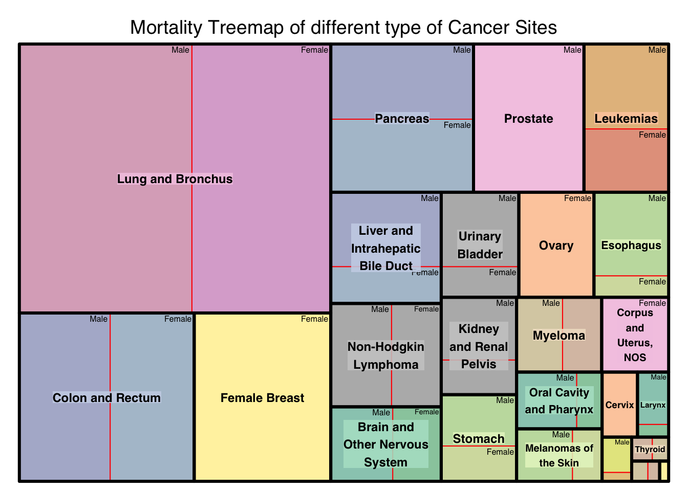
jage_gg1<-treemap(age_gg_data,index=c("SITE","SEX"),vSize="COUNT",type="index",
title="Mortality Treemap of different type of Cancer Sites",
border.col=c("black","red"),
palette="Pastel2",
fontsize.labels=c(9,6),
align.labels=list(
c("center", "center"),
c("right", "top")
),
)
jage_gg1$tm
SITE SEX vSize vColor stdErr vColorValue
1 Brain and Other Nervous System Female 335234 1269 335234 NA
2 Brain and Other Nervous System Male 427831 1326 427831 NA
3 Brain and Other Nervous System <NA> 763065 2595 763065 NA
4 Cervix Female 213459 1146 213459 NA
5 Cervix <NA> 213459 1146 213459 NA
6 Colon and Rectum Female 1312070 1351 1312070 NA
7 Colon and Rectum Male 1416948 1385 1416948 NA
8 Colon and Rectum <NA> 2729018 2736 2729018 NA
9 Corpus and Uterus, NOS Female 464297 1070 464297 NA
10 Corpus and Uterus, NOS <NA> 464297 1070 464297 NA
11 Esophagus Female 148950 680 148950 NA
12 Esophagus Male 578605 1007 578605 NA
13 Esophagus <NA> 727555 1687 727555 NA
14 Female Breast Female 2131713 1427 2131713 NA
15 Female Breast <NA> 2131713 1427 2131713 NA
16 Hodgkin Lymphoma Female 22300 507 22300 NA
17 Hodgkin Lymphoma Male 30281 568 30281 NA
18 Hodgkin Lymphoma <NA> 52581 1075 52581 NA
19 Kidney and Renal Pelvis Female 242377 861 242377 NA
20 Kidney and Renal Pelvis Male 438065 1042 438065 NA
21 Kidney and Renal Pelvis <NA> 680442 1903 680442 NA
22 Larynx Female 36733 451 36733 NA
23 Larynx Male 151162 734 151162 NA
24 Larynx <NA> 187895 1185 187895 NA
25 Leukemias Female 497151 1474 497151 NA
26 Leukemias Male 666520 1582 666520 NA
27 Leukemias <NA> 1163671 3056 1163671 NA
28 Liver and Intrahepatic Bile Duct Female 377447 1076 377447 NA
29 Liver and Intrahepatic Bile Duct Male 761343 1246 761343 NA
30 Liver and Intrahepatic Bile Duct <NA> 1138790 2322 1138790 NA
31 Lung and Bronchus Female 3463424 1339 3463424 NA
32 Lung and Bronchus Male 4302107 1368 4302107 NA
33 Lung and Bronchus <NA> 7765531 2707 7765531 NA
34 Melanomas of the Skin Female 144412 553 144412 NA
35 Melanomas of the Skin Male 271799 606 271799 NA
36 Melanomas of the Skin <NA> 416211 1159 416211 NA
37 Mesothelioma Female 24659 344 24659 NA
38 Mesothelioma Male 96777 443 96777 NA
39 Mesothelioma <NA> 121436 787 121436 NA
40 Myeloma Female 271448 827 271448 NA
41 Myeloma Male 318583 878 318583 NA
42 Myeloma <NA> 590031 1705 590031 NA
43 Non-Hodgkin Lymphoma Female 476322 1144 476322 NA
44 Non-Hodgkin Lymphoma Male 582126 1287 582126 NA
45 Non-Hodgkin Lymphoma <NA> 1058448 2431 1058448 NA
46 Oral Cavity and Pharynx Female 134126 724 134126 NA
47 Oral Cavity and Pharynx Male 315783 1017 315783 NA
48 Oral Cavity and Pharynx <NA> 449909 1741 449909 NA
49 Ovary Female 731683 1221 731683 NA
50 Ovary <NA> 731683 1221 731683 NA
51 Pancreas Female 966936 1091 966936 NA
52 Pancreas Male 994615 1148 994615 NA
53 Pancreas <NA> 1961551 2239 1961551 NA
54 Prostate Male 1517558 976 1517558 NA
55 Prostate <NA> 1517558 976 1517558 NA
56 Stomach Female 246919 1176 246919 NA
57 Stomach Male 358543 1192 358543 NA
58 Stomach <NA> 605462 2368 605462 NA
59 Testis Male 16938 414 16938 NA
60 Testis <NA> 16938 414 16938 NA
61 Thyroid Female 45832 470 45832 NA
62 Thyroid Male 36224 413 36224 NA
63 Thyroid <NA> 82056 883 82056 NA
64 Urinary Bladder Female 220753 706 220753 NA
65 Urinary Bladder Male 535148 843 535148 NA
66 Urinary Bladder <NA> 755901 1549 755901 NA
level x0 y0 w h color
1 2 0.5749978 0.00000000 0.07472981 0.17040506 #99CBAC
2 2 0.4796264 0.00000000 0.09537138 0.17040506 #99CBBD
3 1 0.4796264 0.00000000 0.17010119 0.17040506 #B3E2CD
4 2 0.8974732 0.10115117 0.05452861 0.14870253 #FDCDAC
5 1 0.8974732 0.10115117 0.05452861 0.14870253 #FDCDAC
6 2 0.1398155 0.00000000 0.12946683 0.38496991 #B1C2D1
7 2 0.0000000 0.00000000 0.13981553 0.38496991 #B1B7D1
8 1 0.0000000 0.00000000 0.26928237 0.38496991 #CBD5E8
9 2 0.8968617 0.24985370 0.10313834 0.17100313 #F4CAE4
10 1 0.8968617 0.24985370 0.10313834 0.17100313 #F4CAE4
11 2 0.8849542 0.42085683 0.11504579 0.04918108 #D4DDAD
12 2 0.8849542 0.47003791 0.11504579 0.19104679 #C4DDAD
13 1 0.8849542 0.42085683 0.11504579 0.24022787 #E6F5C9
14 2 0.2692824 0.00000000 0.21034406 0.38496991 #FFF2AE
15 1 0.2692824 0.00000000 0.21034406 0.38496991 #FFF2AE
16 2 0.9678717 0.00000000 0.01825939 0.04639240 #D9C2B1
17 2 0.9430774 0.00000000 0.02479429 0.04639240 #D9CFB1
18 1 0.9430774 0.00000000 0.04305368 0.04639240 #F1E2CC
19 2 0.6497276 0.19815851 0.11606532 0.07932631 #B8B8B8
20 2 0.6497276 0.27748482 0.11606532 0.14337202 #B8B8B8
21 1 0.6497276 0.19815851 0.11606532 0.22269832 #CCCCCC
22 2 0.9520018 0.10115117 0.04799822 0.02907097 #99CBAC
23 2 0.9520018 0.13022214 0.04799822 0.11963156 #99CBBD
24 1 0.9520018 0.10115117 0.04799822 0.14870253 #B3E2CD
25 2 0.8695730 0.66108470 0.13042695 0.14479357 #E4A18C
26 2 0.8695730 0.80587827 0.13042695 0.19412173 #E4BE8C
27 1 0.8695730 0.66108470 0.13042695 0.33891530 #FDCDAC
28 2 0.4796264 0.40677403 0.17010119 0.08429017 #B1C2D1
29 2 0.4796264 0.49106420 0.17010119 0.17002050 #B1B7D1
30 1 0.4796264 0.40677403 0.17010119 0.25431067 #CBD5E8
31 2 0.2657132 0.38496991 0.21391321 0.61503009 #DCAED2
32 2 0.0000000 0.38496991 0.26571321 0.61503009 #DCAEC3
33 1 0.0000000 0.38496991 0.47962642 0.61503009 #F4CAE4
34 2 0.8517843 0.00000000 0.04568886 0.12006634 #D4DDAD
35 2 0.7657929 0.00000000 0.08599137 0.12006634 #C4DDAD
36 1 0.7657929 0.00000000 0.13168023 0.12006634 #E6F5C9
37 2 0.8974732 0.00000000 0.04560420 0.02053993 #E6C98E
38 2 0.8974732 0.02053993 0.04560420 0.08061124 #E5E68E
39 1 0.8974732 0.00000000 0.04560420 0.10115117 #FFF2AE
40 2 0.8365626 0.24985370 0.06029911 0.17100313 #D9C2B1
41 2 0.7657929 0.24985370 0.07076962 0.17100313 #D9CFB1
42 1 0.7657929 0.24985370 0.13106873 0.17100313 #F1E2CC
43 2 0.5731788 0.17040506 0.07654882 0.23636897 #B8B8B8
44 2 0.4796264 0.17040506 0.09355238 0.23636897 #B8B8B8
45 1 0.4796264 0.17040506 0.17010119 0.23636897 #CCCCCC
46 2 0.8582169 0.12006634 0.03925626 0.12978736 #99CBAC
47 2 0.7657929 0.12006634 0.09242398 0.12978736 #99CBBD
48 1 0.7657929 0.12006634 0.13168023 0.12978736 #B3E2CD
49 2 0.7692557 0.42085683 0.11569854 0.24022787 #FDCDAC
50 1 0.7692557 0.42085683 0.11569854 0.24022787 #FDCDAC
51 2 0.4796264 0.66108470 0.21985520 0.16706647 #B1C2D1
52 2 0.4796264 0.82815117 0.21985520 0.17184883 #B1B7D1
53 1 0.4796264 0.66108470 0.21985520 0.33891530 #CBD5E8
54 2 0.6994816 0.66108470 0.17009143 0.33891530 #F4CAE4
55 1 0.6994816 0.66108470 0.17009143 0.33891530 #F4CAE4
56 2 0.6497276 0.00000000 0.11606532 0.08081284 #D4DDAD
57 2 0.6497276 0.08081284 0.11606532 0.11734567 #C4DDAD
58 1 0.6497276 0.00000000 0.11606532 0.19815851 #E6F5C9
59 2 0.9861311 0.00000000 0.01386895 0.04639240 #FFF2AE
60 1 0.9861311 0.00000000 0.01386895 0.04639240 #FFF2AE
61 2 0.9430774 0.04639240 0.03179387 0.05475877 #D9C2B1
62 2 0.9748712 0.04639240 0.02512876 0.05475877 #D9CFB1
63 1 0.9430774 0.04639240 0.05692263 0.05475877 #F1E2CC
64 2 0.6497276 0.42085683 0.11952805 0.07015604 #B8B8B8
65 2 0.6497276 0.49101287 0.11952805 0.17007183 #B8B8B8
66 1 0.6497276 0.42085683 0.11952805 0.24022787 #CCCCCC
$type
[1] "index"
$vSize
[1] "COUNT"
$vColor
[1] NA
$stdErr
[1] "COUNT"
$algorithm
[1] "pivotSize"
$vpCoorX
[1] 0.02812148 0.97187852
$vpCoorY
[1] 0.01968504 0.91031496
$aspRatio
[1] 1.483512
$range
[1] NA
$mapping
[1] NA NA NA
$draw
[1] TRUEOne of the most important aspect before checking the spread of the cancer among age group is to see how the cancer sites affects the population in general amongst them. This graph gives a very valuable information about how the cancer sites fare among themselves in general and how it is spread across gender. Lung and Bronchus based cancer are the most prevalent while Throid cancer affects a very less population. Prostate cancer affects only men while Female breast cancer affects only female, and the visualization proves that by not having any subgroup within the Treemap.
US Cancer vs Census Data grouped by Age Parameter - Join
Before we start to analyse the spread of cancer among age groups , it is pertinent to note the relationship between the age groups and the different sites of cancer. It is also important to check the relationship on how many people get cancer and die from cancer among the age group
To achieve these visualizations, our most important step was to perform an inner join between the USCS and US Census dataset both grouped by Age group. The Year,sex and age group was the common column with which the inner join was carried out. This is necessary because we need to find out what percentage of age group population is affected.
Age_joined<-merge(USCS_Age_all,age_data,by.x = c("AGE","YEAR","SEX"),by.y = c("Age","Year","Sex"))

Age_joined_viz<-Age_joined%>%
  group_by(AGE,SEX,SITE,EVENT_TYPE)%>%
  summarize(Total=sum(COUNT))%>%
  filter(SITE!="All Cancer Sites Combined"&SEX!="Male and Female")
US Cancer vs Census Data grouped by Age Parameter - Analysis
age_gg1<-ggplot(Age_joined_viz,aes(y=Total,axis1=AGE,axis3=SITE,axis2=EVENT_TYPE))+
  geom_alluvium(aes(fill=SEX))+
  geom_stratum()+
  geom_text(stat = "stratum",size=1.8,
            aes(label = after_stat(stratum)))+
  scale_x_discrete(limits = c("SEX", "SITE"), expand = c(.05, .05)) +
  scale_fill_brewer(type = "qual", palette = "Set1")+
  ggtitle("Alluvial relationship between Age groups and cancer sites")
age_gg1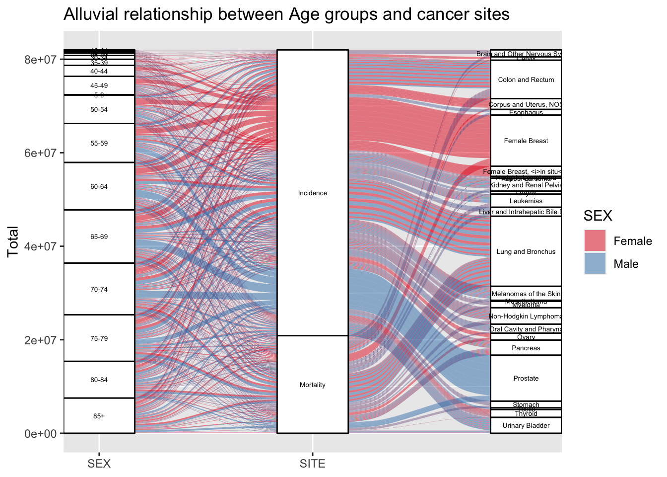
The alluvial flow graph very beautifully captures the flow and relationship between different age groups of the population to the rate of incidence and mortality and also show the relation betweeen these two features with cancer sites. the Age group of 65-69 is most severely affected by cancer. Also interesting and very obvious trend that can be observed over here is that as the age group increases, the rate of cancer also increases. Also to note that Most of the cancer cases are identified and treated , and only one third people die. From the flow relationship diagram, we can see that female breast cancer incidence is far more prevalent than mortality from the same cancer.
Next we want to determine the the spread of cancer across different year group. In order to achieve this, we had to calculate the percentage of population affected each year from cancer cases. Joining the dataset from USCS cancer statistics grouped by age with US census population dataset, helped us to achieve the same. The Count percentage was calculated after getting the population dataset from US census data.
Age_joined_viz2<-Age_joined%>%
  group_by(AGE,SITE,EVENT_TYPE,Population_count,YEAR)%>%
  summarize(Total=sum(COUNT))%>%
  mutate("Count_percent"=Total/Population_count*100)%>%
  ungroup

#head(Age_joined_viz2,30)
area_gg3<-ggplot(Age_joined_viz2%>%filter(EVENT_TYPE=="Incidence"),aes(YEAR,SITE))+
  geom_tile(aes(fill=Count_percent))+
  scale_fill_gradient(high= "blue", low = "white")+
  labs(title="Gradient Heatmap of Cancer Incidence by Year")
ggplotly(area_gg3)
This visualization shows a heat map of Count percentage of population affected by different Cancer sites over a period of two decades. From the graph , we can assume that the year 2017 was the most affected year with new cancer incidences.
area_gg4<-ggplot(Age_joined_viz2%>%filter(EVENT_TYPE=="Mortality"),aes(YEAR,SITE))+
  geom_tile(aes(fill=Count_percent))+
  scale_fill_gradient(low = "white", high = "red") +
  labs(title="Gradient Heatmap of Cancer Mortality by year")
ggplotly(area_gg4)
A similar Heatmap visualization was created for the Cancer mortality cases across two decades and different cancer sites. Most Cancer related deaths happened during the year of 2011 as per the heatmap.
Conclusion
The Cancer dataset was merged and joined with the US population Dataset grouped by Age groups and different states. While visualizing the joined data we were able to answer the questions we started out with . The visualizations aptly answers our questions and shows the spread of cancer among the age group and different states. In conclusion to our findings, living in Utah at a early age might save you from cancer cases historically. There’s no correlation of cancer cases with Age Group or state , we were only concerned about the spread of the cancer cases. As a future work we can look into the correlation between different parameters to determine how likely a person is gonna get affected by cancer.
#save_image(file="AnimeshSenguptaFinalProject.RData")References
[1] National Program of Cancer Registries and Surveillance, Epidemiology, and End Results Program SEER*Stat Database: NPCR and SEER Incidence – U.S. Cancer Statistics Public Use Research Database, 2021 submission (2001–2019), United States Department of Health and Human Services, Centers for Disease Control and Prevention and National Cancer Institute. Released June 2022. Available at www.cdc.gov/cancer/uscs/public-use.
[2]U.S. Census Bureau. “Population Estimates, July 1, 1999-2020 (V2020) – Walla Walla city, WA.” Quick Facts, https://www2.census.gov/programs-surveys/popest/tables/