library(tidyverse)
library(summarytools)
library(lubridate)
library(sf)
library(mapview)
library(leaflet)
library(htmlwidgets)
knitr::opts_chunk$set(echo = TRUE, warning = FALSE, message = FALSE)Final Project
final
tidyverse
summarytools
lubridate
sf
mapview
leaflet
Crime, Drug Usage and Demographics
Introduction
Brooklyn Nine-Nine, which is about a police precinct in New York City, is one of my favourite TV shows. It made me want to learn more about actual crime statistics in the city.
Specifically, this project examines how crime intersects with other social issues. The disparities in arrest rates across demographic groups have been well-documented (Jahn et al., 2022; Schleiden et al., 2020). Past research has also revealed a positive association between crime and drug usage (Pierce et al., 2017).
Research Questions
- What is the demographic profile of those arrested for drug-related crimes? Does it differ from that of general offenders?
- Suppose you were walking through a borough in New York City, and you see syringe litter. Does this necessarily mean that the borough in question is unsafe – or is this merely a bias that we have? In simpler terms: where are syringes likely to be found? Is there an overlap with where drug-related crimes occur?
Crime is operationalized as arrest data (New York Police Department, 2022a; New York Police Department, 2022b), and drug usage as syringe litter data (NYC Parks, 2022a). The data spans from 2017 to 2022. Codebooks are provided here (New York Police Department, 2022a) and here (NYC Parks, 2022b).
Read In Data
# read in arrest datasets.
arrest_historic <- read_csv("~/Desktop/umass/601final/historic.csv",
show_col_types = FALSE,
col_names = c("del", "date", "del", "del", "del", "a_desc", "del", "a_offenselevel", "a_boro", "del", "del", "a_age", "a_sex", "a_race", "del", "del", "a_lat", "a_long", "del"), skip=1) %>%
select(!starts_with("del"))
arrest_ytd <- read_csv("~/Desktop/umass/601final/ytd.csv",
show_col_types = FALSE,
col_names = c("del", "date", "del", "del", "del", "a_desc", "del", "a_offenselevel", "a_boro", "del", "del", "a_age", "a_sex", "a_race", "del", "del", "a_lat", "a_long", "del"), skip=1) %>%
select(!starts_with("del"))
# replace "9" (missing) with NA.
arrest_ytd$a_offenselevel <- na_if(arrest_ytd$a_offenselevel, "9")
# read in syringe dataset.
syringe <- read_csv("~/Desktop/umass/601final/syringe.csv", show_col_types = FALSE, col_names = c("del", "gispropnum", "del", "date", "del", "del", "del", "del", "del", "del", "s_location", "s_groundsyringes", "s_kiosksyringes", "s_totalsyringes", "del", "del", "del", "s_boro", "del", "del", "del", "del", "del"), skip=1) %>%
select(!starts_with("del")) %>%
filter(s_totalsyringes > 0)
# make any implicit missing values explicit.
arrest_historic <- complete(arrest_historic)
arrest_ytd <- complete(arrest_ytd)
syringe <- complete(syringe)
# summarise the 3 datasets.
print(dfSummary(arrest_historic, varnumbers = FALSE, plain.ascii = FALSE, graph.magnif = 0.30, style = "grid", valid.col = FALSE),
method = 'render', table.classes = 'table-condensed')Data Frame Summary
arrest_historic
Dimensions: 5308876 x 9Duplicates: 389555
| Variable | Stats / Values | Freqs (% of Valid) | Graph | Missing | |||||||||||||||||||||||||||||||||||||||||||||||||||||||
|---|---|---|---|---|---|---|---|---|---|---|---|---|---|---|---|---|---|---|---|---|---|---|---|---|---|---|---|---|---|---|---|---|---|---|---|---|---|---|---|---|---|---|---|---|---|---|---|---|---|---|---|---|---|---|---|---|---|---|---|
| date [character] |
|
|
 |
0 (0.0%) | |||||||||||||||||||||||||||||||||||||||||||||||||||||||
| a_desc [character] |
|
|
 |
9169 (0.2%) | |||||||||||||||||||||||||||||||||||||||||||||||||||||||
| a_offenselevel [character] |
|
|
 |
20254 (0.4%) | |||||||||||||||||||||||||||||||||||||||||||||||||||||||
| a_boro [character] |
|
|
 |
8 (0.0%) | |||||||||||||||||||||||||||||||||||||||||||||||||||||||
| a_age [character] |
|
|
 |
17 (0.0%) | |||||||||||||||||||||||||||||||||||||||||||||||||||||||
| a_sex [character] |
|
|
 |
0 (0.0%) | |||||||||||||||||||||||||||||||||||||||||||||||||||||||
| a_race [character] |
|
|
 |
0 (0.0%) | |||||||||||||||||||||||||||||||||||||||||||||||||||||||
| a_lat [numeric] |
|
105327 distinct values |  |
1 (0.0%) | |||||||||||||||||||||||||||||||||||||||||||||||||||||||
| a_long [numeric] |
|
104874 distinct values |  |
1 (0.0%) |
Generated by summarytools 1.0.1 (R version 4.2.1)
2022-09-02
print(dfSummary(arrest_ytd, varnumbers = FALSE, plain.ascii = FALSE, graph.magnif = 0.30, style = "grid", valid.col = FALSE),
method = 'render', table.classes = 'table-condensed')Data Frame Summary
arrest_ytd
Dimensions: 93238 x 9Duplicates: 10143
| Variable | Stats / Values | Freqs (% of Valid) | Graph | Missing | |||||||||||||||||||||||||||||||||||||||||||||||||||||||
|---|---|---|---|---|---|---|---|---|---|---|---|---|---|---|---|---|---|---|---|---|---|---|---|---|---|---|---|---|---|---|---|---|---|---|---|---|---|---|---|---|---|---|---|---|---|---|---|---|---|---|---|---|---|---|---|---|---|---|---|
| date [character] |
|
|
 |
0 (0.0%) | |||||||||||||||||||||||||||||||||||||||||||||||||||||||
| a_desc [character] |
|
|
 |
0 (0.0%) | |||||||||||||||||||||||||||||||||||||||||||||||||||||||
| a_offenselevel [character] |
|
|
 |
1127 (1.2%) | |||||||||||||||||||||||||||||||||||||||||||||||||||||||
| a_boro [character] |
|
|
 |
0 (0.0%) | |||||||||||||||||||||||||||||||||||||||||||||||||||||||
| a_age [character] |
|
|
 |
0 (0.0%) | |||||||||||||||||||||||||||||||||||||||||||||||||||||||
| a_sex [character] |
|
|
 |
0 (0.0%) | |||||||||||||||||||||||||||||||||||||||||||||||||||||||
| a_race [character] |
|
|
 |
0 (0.0%) | |||||||||||||||||||||||||||||||||||||||||||||||||||||||
| a_lat [numeric] |
|
18038 distinct values |  |
0 (0.0%) | |||||||||||||||||||||||||||||||||||||||||||||||||||||||
| a_long [numeric] |
|
18022 distinct values |  |
0 (0.0%) |
Generated by summarytools 1.0.1 (R version 4.2.1)
2022-09-02
print(dfSummary(syringe, varnumbers = FALSE, plain.ascii = FALSE, graph.magnif = 0.30, style = "grid", valid.col = FALSE),
method = 'render', table.classes = 'table-condensed')Data Frame Summary
syringe
Dimensions: 17531 x 7Duplicates: 1704
| Variable | Stats / Values | Freqs (% of Valid) | Graph | Missing | |||||||||||||||||||||||||||||||||||||||||||||||||||||||
|---|---|---|---|---|---|---|---|---|---|---|---|---|---|---|---|---|---|---|---|---|---|---|---|---|---|---|---|---|---|---|---|---|---|---|---|---|---|---|---|---|---|---|---|---|---|---|---|---|---|---|---|---|---|---|---|---|---|---|---|
| gispropnum [character] |
|
|
 |
49 (0.3%) | |||||||||||||||||||||||||||||||||||||||||||||||||||||||
| date [character] |
|
|
 |
0 (0.0%) | |||||||||||||||||||||||||||||||||||||||||||||||||||||||
| s_location [character] |
|
|
|
49 (0.3%) | |||||||||||||||||||||||||||||||||||||||||||||||||||||||
| s_groundsyringes [numeric] |
|
328 distinct values |  |
3284 (18.7%) | |||||||||||||||||||||||||||||||||||||||||||||||||||||||
| s_kiosksyringes [numeric] |
|
110 distinct values |  |
13977 (79.7%) | |||||||||||||||||||||||||||||||||||||||||||||||||||||||
| s_totalsyringes [numeric] |
|
364 distinct values | |
0 (0.0%) | |||||||||||||||||||||||||||||||||||||||||||||||||||||||
| s_boro [character] |
|
|
 |
49 (0.3%) |
Generated by summarytools 1.0.1 (R version 4.2.1)
2022-09-02
#read in shapefile for syringe dataset.
park <- st_read("_data/ParksProperties", quiet = TRUE) %>% select("gispropnum", "geometry")In the code chunk above, all datasets have been loaded, unnecessary columns removed, columns renamed where needed and all missing values labelled NA. Some missing values were labelled “9” in the arrest_ytd dataset and have also been converted to NA.
The arrest_historic dataset contains 5,308,876 rows, while the arrest_ytd dataset contains 93,238 rows. Each row represents a single arrest and associated information (e.g., description of crime, arrest location, demographic profile of suspect). Both have the same 9 columns and only differ in time frame: the arrest_historic dataset contains data from Jan 2006 to Dec 2021, while the arrest_ytd dataset contains data from Jan to Jun 2022.
Some initial observations:
Dangerous drugs are in the list of top 5 offenses in both datasets, highlighting the importance of our research questions.
Arrests seem to occur the least often in Staten Island - it would be interesting to see if this is where the least number of syringes are collected as well.
Black individuals represent almost half of all arrests in both datasets, despite only being ~20% of the population in NYC (U.S. Census Bureau, 2022).
Meanwhile, the syringe dataset contains 17,531 rows and 7 columns. Rows where “total syringes collected = 0” were removed in the read-in, as they are not meaningful for analysis. The dataset ranges from Jan 2017 to Jul 2022. It contains information on syringes collected in NYC, including date, location and number of syringes. Each row does not yet represent a single date/location combination of syringe collection, so it needs to be tidied before descriptives can be interpreted. One initial observation is that no syringes were collected in Brooklyn.
I have also loaded the park shapefile (Department of Parks and Recreation, 2022), which will be used derive location coordinates for the syringe dataset.
Tidy Data
Steps to tidy arrest_historic and arrest_ytd datasets:
Convert date to “date” column type.
Create a separate column, year.
Remove rows before 2017 in the arrest_historic dataset(results in 1,043,535 rows).
Join both datasets into the arrest dataset (93,238 + 1,043,535 = 1,136,773 rows; 9 + 1 = 10 columns).
# change 'date' to date column type.
arrest_historic <- arrest_historic %>% mutate(date = as_date(parse_date_time(date, c('mdy'))))
arrest_ytd <- arrest_ytd %>% mutate(date = as_date(parse_date_time(date, c('mdy'))))# create 'year'.
arrest_historic$"year" <- year(arrest_historic$date)
arrest_ytd$"year" <- year(arrest_ytd$date)
# remove rows before 2017 in arrest_historic.
arrest_historic <- arrest_historic %>% filter(year > 2016)
# join datasets.
arrest <- rbind(arrest_historic, arrest_ytd)
# spell out borough names in full.
arrest$a_boro <- recode(arrest$a_boro, B = 'Bronx', S = 'Staten Island', K = 'Brooklyn', M = 'Manhattan', Q = 'Queens')
# sanity check.
print(dfSummary(arrest, varnumbers = FALSE, plain.ascii = FALSE, graph.magnif = 0.30, style = "grid", valid.col = FALSE),
method = 'render', table.classes = 'table-condensed')Data Frame Summary
arrest
Dimensions: 1136773 x 10Duplicates: 97724
| Variable | Stats / Values | Freqs (% of Valid) | Graph | Missing | |||||||||||||||||||||||||||||||||||||||||||||||||||||||
|---|---|---|---|---|---|---|---|---|---|---|---|---|---|---|---|---|---|---|---|---|---|---|---|---|---|---|---|---|---|---|---|---|---|---|---|---|---|---|---|---|---|---|---|---|---|---|---|---|---|---|---|---|---|---|---|---|---|---|---|
| date [Date] |
|
2007 distinct values |  |
0 (0.0%) | |||||||||||||||||||||||||||||||||||||||||||||||||||||||
| a_desc [character] |
|
|
 |
2031 (0.2%) | |||||||||||||||||||||||||||||||||||||||||||||||||||||||
| a_offenselevel [character] |
|
|
 |
8538 (0.8%) | |||||||||||||||||||||||||||||||||||||||||||||||||||||||
| a_boro [character] |
|
|
 |
0 (0.0%) | |||||||||||||||||||||||||||||||||||||||||||||||||||||||
| a_age [character] |
|
|
 |
0 (0.0%) | |||||||||||||||||||||||||||||||||||||||||||||||||||||||
| a_sex [character] |
|
|
 |
0 (0.0%) | |||||||||||||||||||||||||||||||||||||||||||||||||||||||
| a_race [character] |
|
|
 |
0 (0.0%) | |||||||||||||||||||||||||||||||||||||||||||||||||||||||
| a_lat [numeric] |
|
93984 distinct values |  |
0 (0.0%) | |||||||||||||||||||||||||||||||||||||||||||||||||||||||
| a_long [numeric] |
|
93555 distinct values |  |
0 (0.0%) | |||||||||||||||||||||||||||||||||||||||||||||||||||||||
| year [numeric] |
|
|
 |
0 (0.0%) |
Generated by summarytools 1.0.1 (R version 4.2.1)
2022-09-02
The sanity check demonstrates that steps 1 to 4 are complete.
Steps to tidy the syringe dataset:
Convert date to “date” type.
Sum syringe count values in the syringe dataset into 1 row per date/location combination.
Extract latitude and longitude columns from park shapefile and convert them into a dataframe.
Combine that dataframe with the syringe dataset (will produce <17,531 rows and 9 columns).
# remove timestamp from 'date'.
syringe$date <- str_remove(syringe$date, "12:00:00 AM")
# convert 'date' to date column type.
syringe <- syringe %>% mutate(date = as_date(parse_date_time(date, c('mdy'))))
# sum syringe count values into 1 row per date/location combo.
syringe <- syringe %>%
group_by(s_location, date, gispropnum, s_boro) %>%
summarise(across(contains("syringes"), ~sum(.x, na.rm = TRUE)))
# extract latitude and longitude from park shapefile into park_ll.
sf_use_s2(FALSE)
park_ll <- st_coordinates(st_centroid(park$geometry))
# convert park and park_ll to dataframes.
park_ll <- as_tibble(park_ll)
park <- as_tibble(park)
# remove multipolygon column from park.
park <- select(park, -2)
# combine park and park_ll.
park <- cbind(park, park_ll)
# rename long and lat columns in park.
park <- rename(park, "s_long" = "X", "s_lat" = "Y")
# combine park and syringe.
syringe <- syringe %>%
left_join(park, by = "gispropnum")
# sanity check.
class(syringe$date)[1] "Date"colnames(syringe)[1] "s_location" "date" "gispropnum" "s_boro"
[5] "s_groundsyringes" "s_kiosksyringes" "s_totalsyringes" "s_long"
[9] "s_lat" dim(syringe)[1] 9143 9The sanity check shows that steps 1 to 3 are complete. For now, the basic tidying is complete. Further transformations will be required for each visualization.
Analysis: Question 1
To recap, this is my first research question:
Question 1
What is the demographic profile of those arrested for drug-related crimes? Does it differ from that of general offenders?
Age, sex and race data are available in the arrest dataset. We can combine them into 1 column to create demographic profiles, then make bar graphs.
# combine demographics into 1 column.
arrest <- arrest %>%
unite(demo, a_race, a_sex, a_age, sep = "_", remove = FALSE, na.rm = TRUE)
# bar graph of top demographics for all arrests.
arrest %>%
filter(!is.na(demo)) %>%
count(demo) %>%
slice_max(n, n = 5) %>%
ggplot(aes(x = reorder(demo,-n/1136773*100), y = n/1136773 * 100, fill = demo)) +
geom_col(stat="identity") +
theme_minimal() +
labs(title = "Figure 1.1 Top Demographic Profiles: All Arrests, NYC (01/2017-06/2022)", x = "Profile", y = "Percent") +
geom_text(aes(label=sprintf("%0.2f", ..y..)), position=position_dodge(width=0.9), vjust=-0.25, size=3) +
theme(axis.text.x=element_text(angle=90,hjust=1))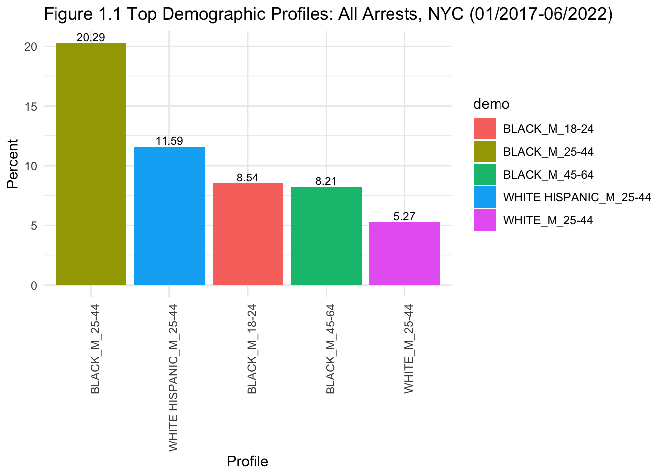
# bar graph of top demographics for drug-related arrests.
arrest %>%
filter(a_desc == "DANGEROUS DRUGS") %>%
filter(!is.na(demo)) %>%
count(demo) %>%
slice_max(n, n = 5) %>%
ggplot(aes(x = reorder(demo,-n/129285*100), y = n/129285 * 100, fill = demo)) +
geom_col(stat="identity") +
theme_minimal() +
labs(title = "Figure 1.2 Top Demographic Profiles: Drug-Related Arrests, NYC (01/2017-06/2022)", x = "Profile", y = "Percent") +
geom_text(aes(label=sprintf("%0.2f", ..y..)), position=position_dodge(width=0.9), vjust=-0.25, size=3) +
theme(axis.text.x=element_text(angle=90,hjust=1))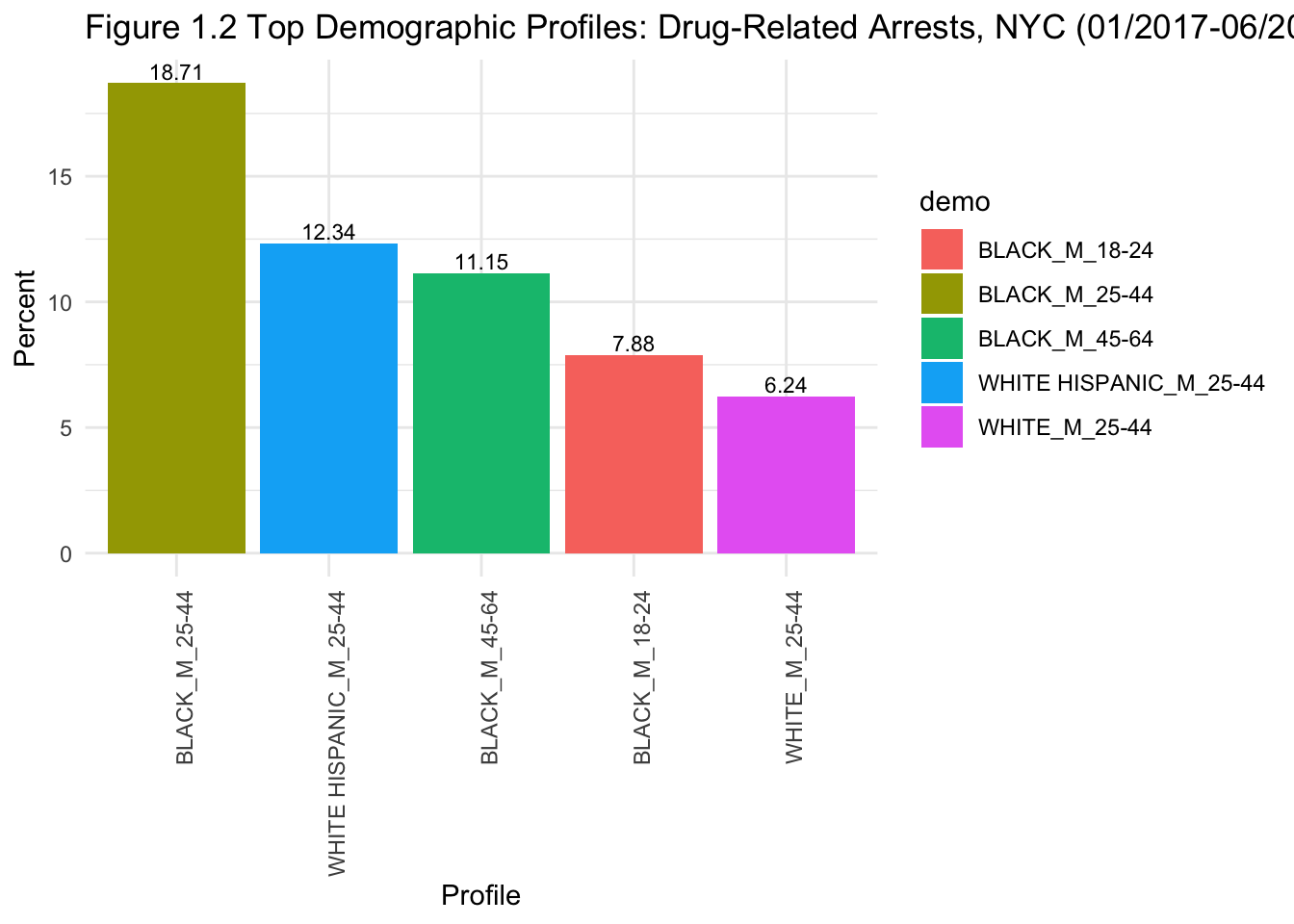
# bar graph of top demographics for drug-related felonies.
arrest %>%
filter(a_desc == "DANGEROUS DRUGS") %>%
filter(a_offenselevel == "F") %>%
filter(!is.na(demo)) %>%
count(demo) %>%
slice_max(n, n = 5) %>%
ggplot(aes(x = reorder(demo,-n/48018*100), y = n/48018*100, fill = demo)) +
geom_col(stat="identity") +
theme_minimal() +
labs(title = "Figure 1.3 Top Demographic Profiles: Drug Felonies, NYC (01/2017-06/2022)", x = "Profile", y = "Percent") +
geom_text(aes(label=sprintf("%0.2f", ..y..)), position=position_dodge(width=0.9), vjust=-0.25, size=3) +
theme(axis.text.x=element_text(angle=90,hjust=1))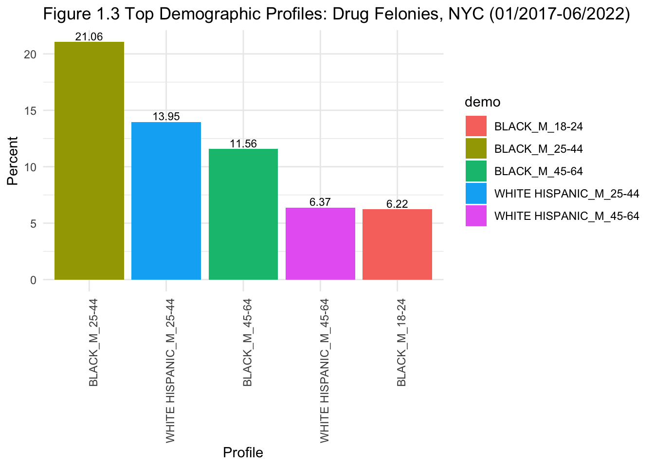
# bar graph of top demogaphics for drug-related misdemeanours.
arrest %>%
filter(a_desc == "DANGEROUS DRUGS") %>%
filter(a_offenselevel == "M") %>%
filter(!is.na(demo)) %>%
count(demo) %>%
slice_max(n, n = 5) %>%
ggplot(aes(x = reorder(demo,-n/81267*100), y = n/81267*100, fill = demo)) +
geom_col(stat="identity") +
theme_minimal() +
labs(title = "Figure 1.4 Top Demographic Profiles: Drug Misdemeanours, NYC (01/2017-06/2022)", x = "Profile", y = "Percent") +
geom_text(aes(label=sprintf("%0.2f", ..y..)), position=position_dodge(width=0.9), vjust=-0.25, size=3) +
theme(axis.text.x=element_text(angle=90,hjust=1))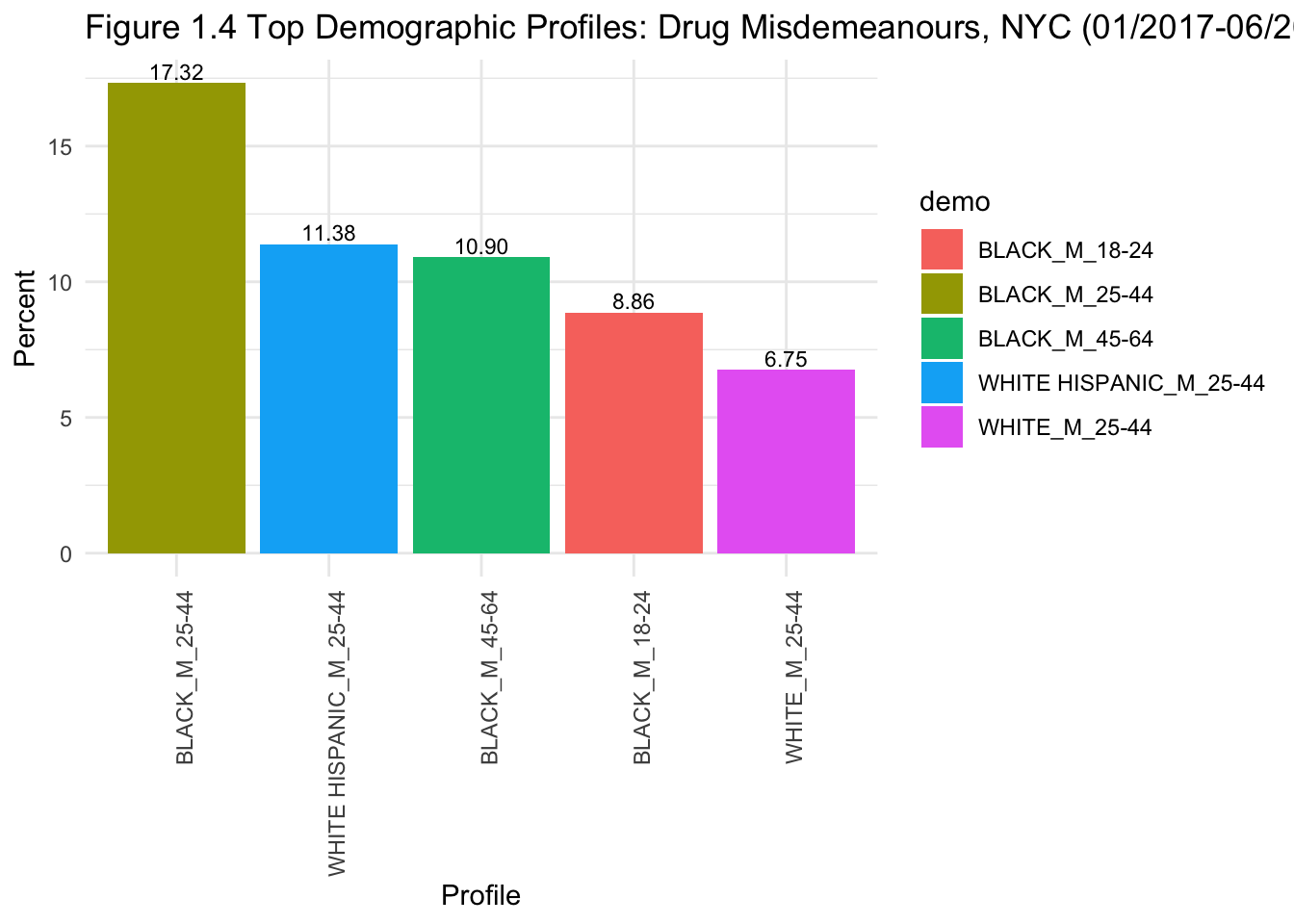
In the above graphs, proportions are calculated based on the subset examined in each graph (e.g., top demographics profiles for drug-related felonies are shown as a proportion of everyone who committed drug-related felonies).
Figures 1.1 and 1.2 show that the top 5 demographic profiles are the same for (1) all arrests and (2) drug-related arrests (except for a switch in order at the 3rd and 4th positions). This somewhat answers our research question:
Question 1
When comparing all arrests and drug-related arrests, the top five demographic profiles of offenders seem to be largely similar. They were all male. Age group varies based on ethnicity: black men aged 18 to 64 are all quite likely to be arrested, although the likelihood was greater for black men aged 25-44. For white Hispanic and white men, arrests were concentrated in the 25-44 age group.
Figures 1.3 and 1.4 help to differentiate the top profiles of those being arrested for drug-related felonies vs. misdemeanours. From the graphs, we can see a change in the top 5 profiles for drug-related felonies: they are all black and white Hispanic men. However, when looking at drug-related misdemeanours, white men are also included. Hence, black and Hispanic men may be more likely to be arrested for drug-related felonies. This shows some evidence of profiling in these arrests, and also aligns with my initial observation that black individuals seem to be overrepresented in arrests in NYC.
# create new dataset for chi-square test (all arrests).
chi_square_all <- arrest %>%
filter(!is.na(demo)) %>%
filter(demo == "BLACK_M_18-24" | demo == "BLACK_M_25-44" | demo == "BLACK_M_45-64" | demo == "WHITE HISPANIC_M_25-44" | demo == "WHITE_M_25-44")
# run chi-square test (all arrests).
chisq.test(x = table(chi_square_all$demo))
Chi-squared test for given probabilities
data: table(chi_square_all$demo)
X-squared = 140432, df = 4, p-value < 2.2e-16# create new dataset for chi-square test (drug-related arrests).
chi_square_drugs <- arrest %>%
filter(!is.na(demo)) %>%
filter(!is.na(a_desc)) %>%
filter(a_desc == "DANGEROUS DRUGS") %>%
filter(demo == "BLACK_M_18-24" | demo == "BLACK_M_25-44" | demo == "BLACK_M_45-64" | demo == "WHITE HISPANIC_M_25-44" | demo == "WHITE_M_25-44")
# run chi-square test (drug-related arrests).
chisq.test(x = table(chi_square_drugs$demo))
Chi-squared test for given probabilities
data: table(chi_square_drugs$demo)
X-squared = 10707, df = 4, p-value < 2.2e-16I ran two chi-square tests to check for significant differences across the frequencies of the top 5 profiles - one for all arrests, one for just drug-related arrests. Both tests revealed significant differences between the top 5 demographic profiles for (1) all arrests, 𝜒2 (4) = 140432, p < .001, and (2) drug-related arrests, 𝜒2 (4) = 10707, p < .001. Instead of doing post-hoc tests, this is where the bar graphs come in handy. They clearly show that the bar for black men aged 25-44 is substantively taller than the bars for the other 4 groups.
Additional Analysis: Question 1
Doing the above analysis also made me interested in exploring two related questions:
How did the proportion of drug-related arrests change over time?
Within drug-related arrests, how did the proportions of each demographic variable (age, sex, race) change over time?
# keep only the top 3 levels of a_desc.
arrest$a_desc <- fct_lump_n(arrest$a_desc, 3, other_level="Other")
# change year to a factor variable, so that i can plot it.
arrest$year <- as.factor(arrest$year)
# stacked bar graph for offense type.
arrest %>% filter(!is.na(a_desc)) %>%
ggplot() +
geom_bar(mapping = aes(x = year, y=..count.., fill=a_desc), position="fill") +
theme_minimal() +
labs(title = "Figure 1.5 Different Arrest Types in NYC (01/2017-06/2022)", x = "Year", y = "Percent") +
scale_y_continuous(labels = scales::percent) +
theme(axis.text.x=element_text(angle=90,hjust=1)) 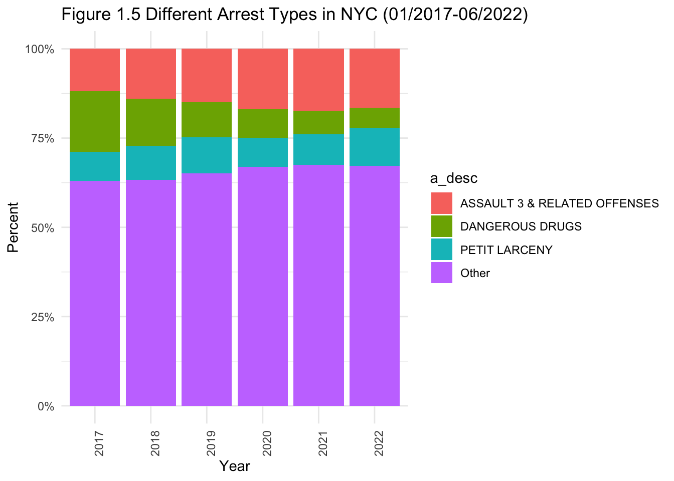
# stacked bar graph for age of drug-related offenders.
arrest %>% filter(a_desc == "DANGEROUS DRUGS") %>%
filter(!is.na(a_age)) %>%
ggplot() +
geom_bar(mapping = aes(x = year, fill=a_age), position="fill") +
theme_minimal() +
labs(title = "Figure 1.6 Age Composition of Drug Arrests in NYC (01/2017-06/2022)", x = "Year", y = "Percent") +
scale_y_continuous(labels = scales::percent) +
theme(axis.text.x=element_text(angle=90,hjust=1))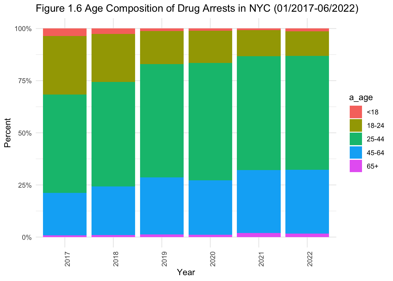
# stacked bar graph for race of drug-related offenders.
arrest %>% filter(a_desc == "DANGEROUS DRUGS") %>%
filter(!is.na(a_race)) %>%
ggplot() +
geom_bar(mapping = aes(x = year, fill=a_race), position="fill") +
theme_minimal() +
labs(title = "Figure 1.7 Race Composition of Drug Arrests in NYC (01/2017-06/2022)", x = "Year", y = "Percent") +
scale_y_continuous(labels = scales::percent) +
theme(axis.text.x=element_text(angle=90,hjust=1))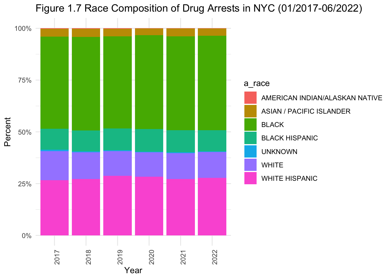
# stacked bar graph for sex of drug-related offenders.
arrest %>% filter(a_desc == "DANGEROUS DRUGS") %>%
filter(!is.na(a_sex)) %>%
ggplot() +
geom_bar(mapping = aes(x = year, fill=a_sex), position="fill") +
theme_minimal() +
labs(title = "Figure 1.8 Sex Composition of Drug Arrests in NYC (01/2017-06/2022)", x = "Year", y = "Percent") +
scale_y_continuous(labels = scales::percent) +
theme(axis.text.x=element_text(angle=90,hjust=1))
- Figure 1.5 shows that the proportion of drug-related arrests has shrunk with time. Although it was a part of the top 3 reasons for arrests, it is definitely on a downward trend.
- Some observations when looking at demographics within drug-related arrests (Figures 1.6 to 1.8):
Men represent the overwhelming majority of drug-related arrests.
Black and black Hispanic individuals make up roughly half of drug-related arrests.
The proportion of those aged 25-64 arrested for drug-related crimes is on the rise.
Analysis: Question 2
To recap, this is my second research question:
Question 2
Suppose you were walking through a borough in New York City, and you see syringe litter. Does this necessarily mean that the borough in question is unsafe – or is this merely a bias that we have? In simpler terms: where are syringes likely to be found? Is there an overlap with where drug-related crimes occur?
Before answering this question, I will generate graphs of how the numbers of drug-related arrests and syringes collected have changed from 2017 to 2021 (since only half of 2022 has occurred).
# counts of syringes.
syringe$"year" <- year(syringe$date)
syringe_count <- syringe %>%
select(year, s_totalsyringes, s_kiosksyringes, s_groundsyringes) %>%
filter(year != 2022) %>%
pivot_longer(contains("syringes"), names_to="syringetype", values_to="count") %>%
group_by(year, syringetype) %>%
summarise(sum = sum(count))
# changing syringetype to factor.
syringe_count$syringetype <- as.factor(syringe_count$syringetype)
# plot syringe count over time.
syringe_count %>%
ggplot(aes(x=year, y=sum, color=syringetype, group=syringetype)) +
geom_line() +
geom_point() +
theme_minimal() +
labs(title = "Figure 2.1 Syringes Collected in NYC (2017-2021)", x = "Year", y = "Number of Syringes") +
geom_text(aes(label=..y..), position=position_dodge(width=0.9), vjust=-0.75, size=3) +
theme(axis.text.x=element_text(angle=90,hjust=1))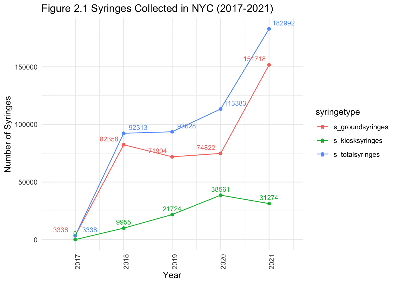
# plot drug-related arrests over time.
arrest %>%
filter(a_desc == "DANGEROUS DRUGS") %>%
select(year) %>%
filter(year != 2022) %>%
count(year) %>%
ggplot(aes(year, n, na.rm = TRUE, group = 1)) +
geom_line() +
geom_point() +
theme_minimal() +
labs(title = "Figure 2.2 Drug-Related Arrests in NYC (2017-2021)", x = "Year", y = "Number of Arrests") +
geom_text(aes(label=..y..), position=position_dodge(width=0.9), vjust=-0.75, size=3) +
theme(axis.text.x=element_text(angle=90,hjust=1))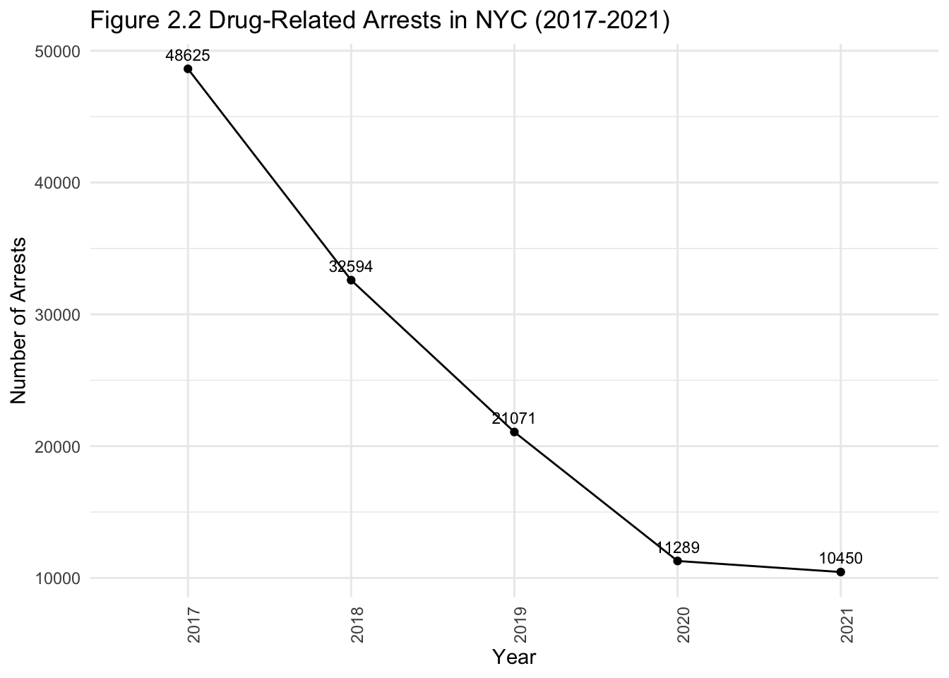
Figure 2.1 shows that syringe litter has gone up with time, and the introduction of kiosks has not been particularly effective.
Meanwhile, Figure 2.2 shows that the number of drug-related arrests has been dropping (as seen in our stacked bar graphs earlier). This is useful in partly answering our research question. In 2022, based on the trends since 2017, someone walking through NYC is probably likely to see syringe litter. However, this may not necessarily mean drug-related crime is high. We can verify this by visualizing dot maps of syringe litter and drug-related arrests.
For the maps, I tested the packages ggmap and mapview. However, the arrest dataset is too large for either package to load the map successfully. I decided to create a new dataframe with the number of arrests in each borough and load that instead. I used mapview, because you can zoom in and out of each borough. The first map shows syringes, while the second shows drug-related arrests.
# visualise syringe using mapview.
syringe %>%
filter(!is.na(s_long)) %>%
filter(!is.na(s_lat)) %>%
filter(!is.na(s_boro)) %>%
group_by(s_boro) %>%
mapview(xcol = "s_long", ycol = "s_lat", crs = 4326, grid = FALSE, layer.name = "Figure 2.3 Syringes by Borough (2017-2022)", at = "s_boro", zcol = "s_boro", legend = TRUE)# creating arrest_map.
arrest_map <- arrest %>%
filter(a_desc == "DANGEROUS DRUGS") %>%
count(a_boro)
arrest_map$lat <-c(40.84567, 40.67908, 40.78322, 40.72955, 40.58098)
arrest_map$long <- c(-73.86136, -73.94672, -73.97198, -73.79636, -74.15237)
# visualisation of arrest_map using mapview.
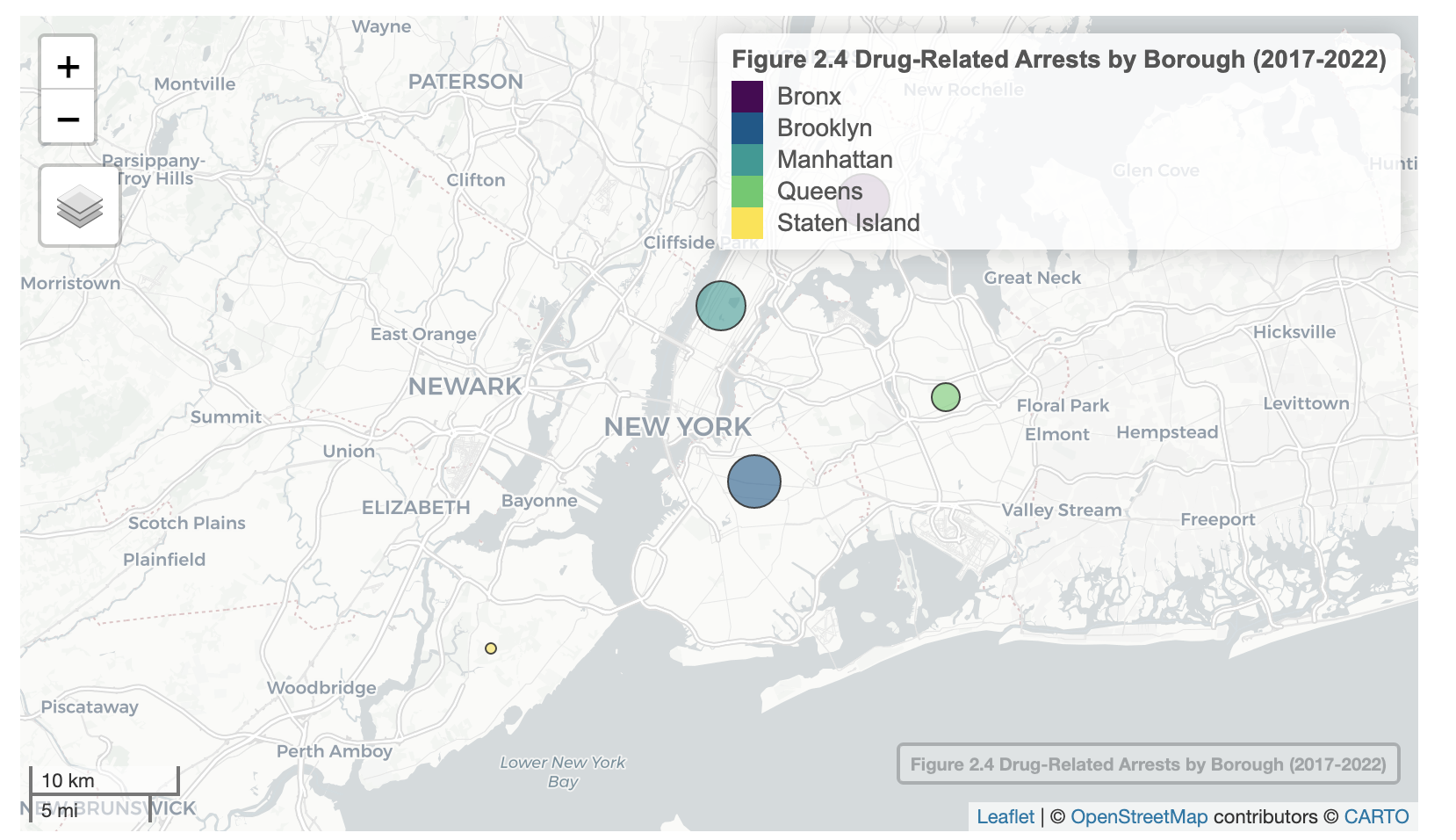
arrest_map %>%
mapview(xcol = "long", ycol = "lat", crs = 4326, grid = FALSE, cex = "n", layer.name = "Figure 2.4 Drug-Related Arrests by Borough (2017-2022)", at = "a_boro", zcol = "a_boro", legend = TRUE)Figure 2.3 and Figure 2.4 confirm what I suspected. From 2017 to 2022, a large number of drug-related arrests occurred in Brooklyn (is this why Brooklyn Nine-Nine is based in Brooklyn?), as denoted by the large size of the circle. The Bronx and Manhattan had a lot of drug-related arrests too. However, the vast majority of syringes seem to be collected from the Bronx. Staten Island seems to have the lowest drug-related crime and drug usage (but this may partly be due to its distance from the city centre). I will generate bar graphs to further verify this.
# drug-related arrests in different boroughs.
arrest %>% filter(a_desc == "DANGEROUS DRUGS") %>%
ggplot(aes(x = a_boro)) +
geom_bar(aes(y=(..count..)/sum(..count..))) +
theme_minimal() +
labs(title = "Figure 2.5 Drug Offenders in NYC Boroughs (01/2017-06/2022)", x = "Borough", y = "Percent of Drug Offenders") +
theme(axis.text.x=element_text(angle=90,hjust=1)) + scale_y_continuous(labels = scales::percent)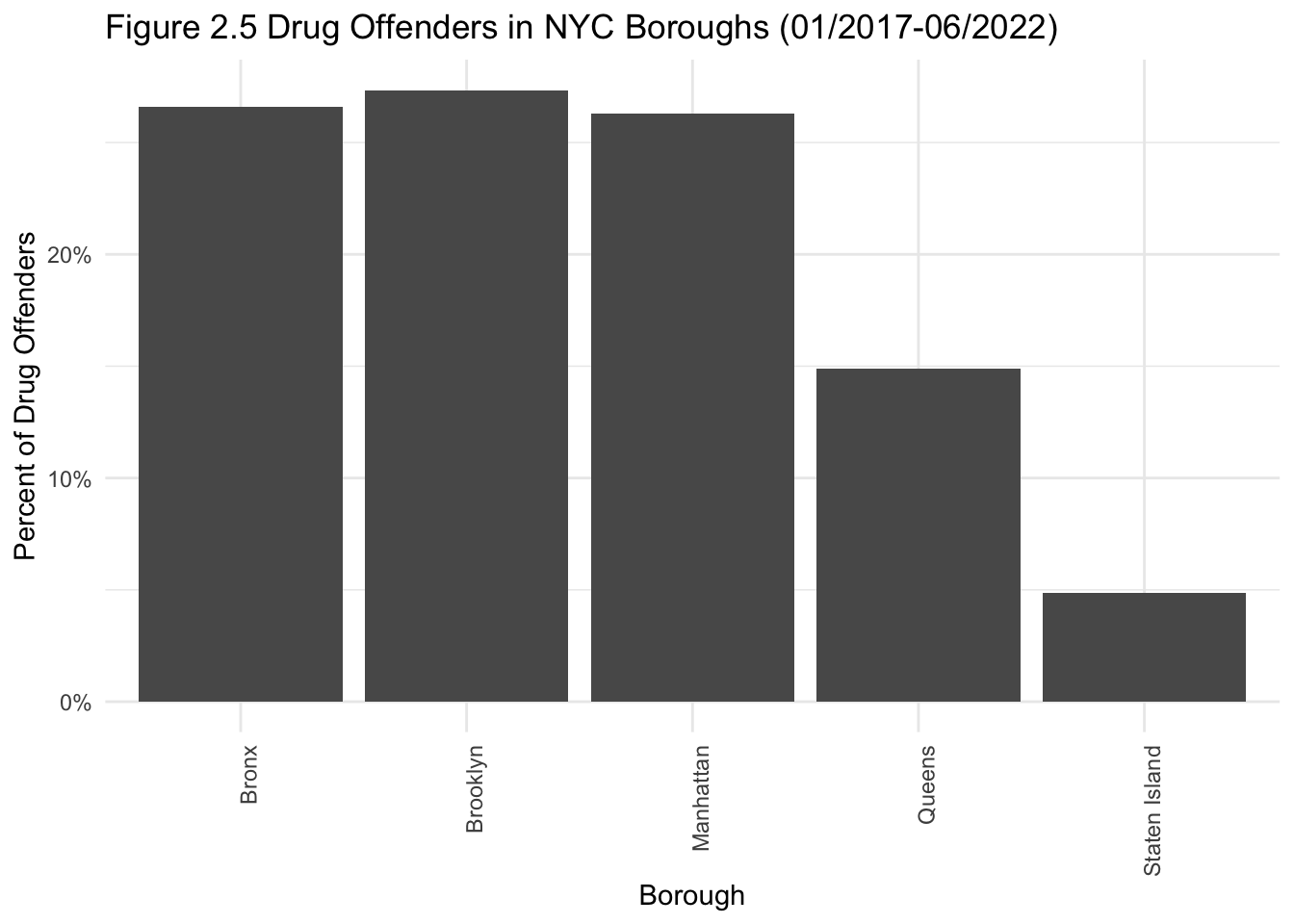
# syringes in different boroughs.
syringe %>%
filter(!is.na(s_boro)) %>%
ggplot(aes(x = s_boro)) +
geom_bar(aes(y=(..count..)/sum(..count..))) +
theme_minimal() +
labs(title = "Figure 2.6 Syringes Collected in NYC Boroughs (01/2017-06/2022)", x = "Borough", y = "Percent of Syringes Collected") + scale_y_continuous(labels = scales::percent) +
theme(axis.text.x=element_text(angle=90,hjust=1)) 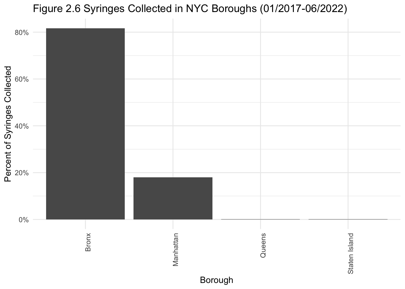
The bar graphs provide more nuance. The percent difference in syringes collected between the Bronx and the other boroughs is massive, with no syringes found in Brooklyn at all. However, drug-related arrests were somewhat equally split between the Bronx, Brooklyn and Manhattan. Going back to my research question, seeing a syringe on the ground does not necessarily mean that the borough in question has a lot of drug-related arrests.
Discussion
Although I began this project with specific research questions, my analysis was somewhat exploratory, as I thought of different ways to extend my main research questions.
Tidying took the most time, and ranged from column manipulation to joins. The most challenging part of this project was learning more about the structure of shapefiles, and how to extract coordinates from multipolygon objects. Although just a few lines of code were required for this, understanding how to do it took a lot of time and practice.
The first research question aimed to examine if demographic profiles of drug-related offenders differed from those of all offenders. They were fairly similar, but profiling became more evident when comparing drug-related felonies vs. misdemeanours (black and Hispanic men were more likely to be arrested for felonies). Further, although drug-related arrests shrunk as a proportion of all arrests over time, demographic profiles of drug-related offenders largely stayed the same.
As a Psychology major in undergrad, I am familiar with using statistical tests to interpret data. Working on this question challenged my assumptions that statistical tests are the “best” way to work with data. Although I did run chi-squares, their results were much easier to interpret when supplemented with bar graphs.
The second research question investigated whether drug-related arrests and syringe litter were positively correlated in terms of location. To answer this question, I generated maps of arrests and syringe litter, and checked if both variables followed the same trajectory over time. They did not have similar patterns over time: drug-related arrests were decreasing, while syringe litter seemed to be increasing. Boroughs where drug-related arrests were happening were not necessarily the same places where drug users lived (except for the Bronx, which is already known to be fairly unsafe in popular culture).
Working on this project has made me question traditional notions of “safety”. Hopefully, the findings allow us to be more empathetic to both drug users and those arrested for drug-related crimes. Structural inequalities often prevent people from seeking help from substance issues, and enable others to become involved in drug-related crimes.
Reflection
I remember finding these datasets and thinking that I was just going to work on arrest (year to date) data and syringe collection data…only to load the syringe collection data and realise that it had datapoints from 2017 onwards. Thus began the journey of reading in a historic arrest dataset with more rows of data than I had ever worked with in my life. This was daunting, given that I had no coding experience. My goal was to push myself out of my comfort zone, and to work with data that I was not already familiar with. This project has challenged my fears and made me more confident in my abilities.
There were some decisions I could have approached differently. For example, when I could not load my arrest dataset into the map of New York City, I decided to just compress it into 1 data point per borough and load that instead. This was sufficient to answer my research question, but I would have grappled with it for longer (if not for time constraints).
Conclusion
Related work in the future can examine the motivations of drug users and those involved in drug-related crimes. This may provide an additional layer of knowledge to the visualizations generated. It would also be useful to look at more data on the usage of syringe exchange kiosks over time, and public perceptions of these kiosks. This would help in understanding why their uptake has been so low.
Bibliography
Department of Parks and Recreation. (2022). Parks Properties. NYC Open Data. Retrieved from https://data.cityofnewyork.us/Recreation/Parks-Properties/enfh-gkve.
Jahn, J., Simes, J., Cowger, T., & Davis, B. (2022). Racial Disparities in Neighborhood Arrest Rates during the COVID-19 Pandemic. Journal Of Urban Health, 99(1), 67-76.
New York Police Department. (2022). NYPD Arrest Data (Year to Date). NYC Open Data. Retrieved from https://data.cityofnewyork.us/Public-Safety/NYPD-Arrest-Data-Year-to-Date-/uip8-fykc.
New York Police Department. (2022). NYPD Arrests Data (Historic). NYC Open Data. Retrieved from https://data.cityofnewyork.us/Public-Safety/NYPD-Arrests-Data-Historic-/8h9b-rp9u.
NYC Parks. (2022). NYC Parks Syringe Litter Data Dictionary and UserGuide. Google Docs. Retrieved from https://docs.google.com/spreadsheets/d/1VSUqd1peSc-4D2XnBZNiLdxa0Jg4z62D/edit#gid=150342678.
NYC Parks. (2022). Summary of Syringe Data in NYC Parks. NYC Open Data. Retrieved from https://data.cityofnewyork.us/Public-Safety/Summary-of-Syringe-Data-in-NYC-Parks/t8xi-d5wb.
Pierce, M., Hayhurst, K., Bird, S., Hickman, M., Seddon, T., Dunn, G., & Millar, T. (2017). Insights into the link between drug use and criminality: Lifetime offending of criminally-active opiate users. Drug And Alcohol Dependence, 179, 309-316.
R Core Team. (2022). R: A language and environment for statistical computing. R Foundation for Statistical Computing.
Schleiden, C., Soloski, K., Milstead, K., & Rhynehart, A. (2020). Racial Disparities in Arrests: A Race Specific Model Explaining Arrest Rates Across Black and White Young Adults. Child And Adolescent Social Work Journal, 37(1), 1-14.
U.S. Census Bureau. (2022). U.S. Census Bureau QuickFacts: New York City, New York. Census Bureau QuickFacts. Retrieved from https://www.census.gov/quickfacts/newyorkcitynewyork.
Wickham, H., & Grolemund, G. (2017). R for Data Science: Import, Tidy, Transform, Visualize, and Model Data (1st ed.). O’Reilly Media.
Appendix (See Below)
Figure 2.3
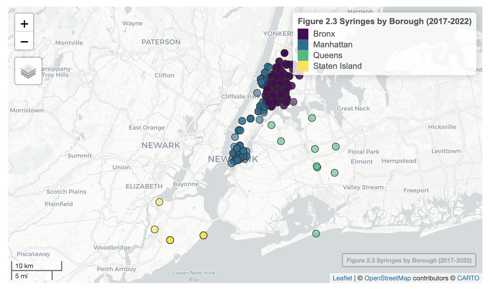
Figure 2.4