library(tidyverse)
library(ggplot2)

knitr::opts_chunk$set(echo = TRUE, warning=FALSE, message=FALSE)
Challenge 5 Instructions
challenge_5
railroads
cereal
air_bnb
pathogen_cost
australian_marriage
public_schools
usa_hh
Introduction to Visualization
Challenge Overview
Today’s challenge is to:
- read in a data set, and describe the data set using both words and any supporting information (e.g., tables, etc)
- tidy data (as needed, including sanity checks)
- mutate variables as needed (including sanity checks)
- create at least two univariate visualizations
- try to make them “publication” ready
- Explain why you choose the specific graph type
- Create at least one bivariate visualization
- try to make them “publication” ready
- Explain why you choose the specific graph type
R Graph Gallery is a good starting point for thinking about what information is conveyed in standard graph types, and includes example R code.
(be sure to only include the category tags for the data you use!)
Read in data
Read in one (or more) of the following datasets, using the correct R package and command.
- cereal ⭐
- pathogen cost ⭐
- Australian Marriage ⭐⭐
- AB_NYC_2019.csv ⭐⭐⭐
- railroads ⭐⭐⭐
- Public School Characteristics ⭐⭐⭐⭐
- USA Households ⭐⭐⭐⭐⭐
library(readr)
AB_NYC <- read_csv("_data/AB_NYC_2019.csv")
Briefly describe the data
Tidy Data (as needed)
Is your data already tidy, or is there work to be done? Be sure to anticipate your end result to provide a sanity check, and document your work here.
head(AB_NYC)# A tibble: 6 × 16
id name host_id host_…¹ neigh…² neigh…³ latit…⁴ longi…⁵ room_…⁶ price
<dbl> <chr> <dbl> <chr> <chr> <chr> <dbl> <dbl> <chr> <dbl>
1 2539 Clean & q… 2787 John Brookl… Kensin… 40.6 -74.0 Privat… 149
2 2595 Skylit Mi… 2845 Jennif… Manhat… Midtown 40.8 -74.0 Entire… 225
3 3647 THE VILLA… 4632 Elisab… Manhat… Harlem 40.8 -73.9 Privat… 150
4 3831 Cozy Enti… 4869 LisaRo… Brookl… Clinto… 40.7 -74.0 Entire… 89
5 5022 Entire Ap… 7192 Laura Manhat… East H… 40.8 -73.9 Entire… 80
6 5099 Large Coz… 7322 Chris Manhat… Murray… 40.7 -74.0 Entire… 200
# … with 6 more variables: minimum_nights <dbl>, number_of_reviews <dbl>,
# last_review <date>, reviews_per_month <dbl>,
# calculated_host_listings_count <dbl>, availability_365 <dbl>, and
# abbreviated variable names ¹host_name, ²neighbourhood_group,
# ³neighbourhood, ⁴latitude, ⁵longitude, ⁶room_type
# ℹ Use `colnames()` to see all variable namesAre there any variables that require mutation to be usable in your analysis stream? For example, do you need to calculate new values in order to graph them? Can string values be represented numerically? Do you need to turn any variables into factors and reorder for ease of graphics and visualization?
Document your work here.
price_analysis <- AB_NYC %>% select(neighbourhood_group,room_type,price,minimum_nights)Univariate Visualizations
Since this was a single variable I wanted to look at, I wanted to see which neighborhood had the largest amount of Units.
ggplot(price_analysis, mapping = aes(x = neighbourhood_group)) +
  geom_bar(fill = "red") +
  labs(title = "# of Unit Listings per Neighboorhood", x = "Neighboorhood", y = "Number of Units")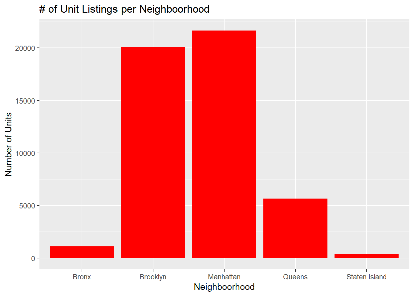
Bivariate Visualization(s)
Any additional comments?
I Kinda did a a Tri-Variate Visualization. I wanted to find the prices of all Room Types by Neighborhoods.
ggplot(price_analysis, mapping = aes(x = room_type,y=price,color="room_type")) +
  geom_point() +
  facet_wrap(vars(neighbourhood_group)) +
  labs(title = "Room Type by Neighbourhoods", x = "Room Type", y = "Count")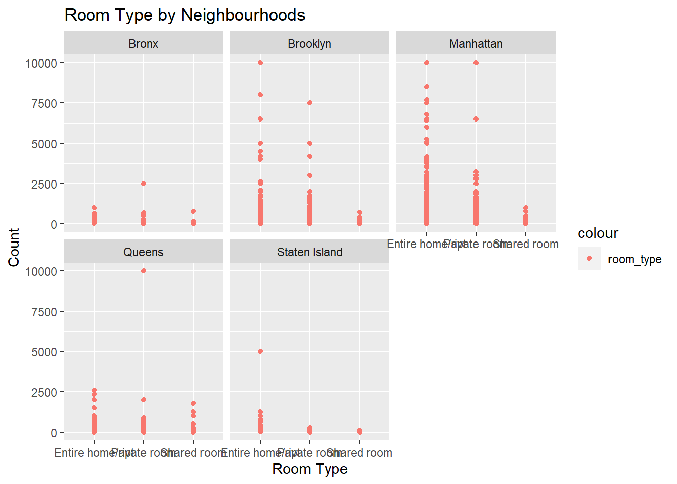
Also just wanted to do a table analysis of Room Type and Neighborhood Group.
table(price_analysis$neighbourhood_group,price_analysis$room_type)
                Entire home/apt Private room Shared room
  Bronx                     379          652          60
  Brooklyn                 9559        10132         413
  Manhattan               13199         7982         480
  Queens                   2096         3372         198
  Staten Island             176          188           9
I also did a Table Function to see Chi-Square Contribution.
library(gmodels)
CrossTable(price_analysis$neighbourhood_group,price_analysis$room_type)
   Cell Contents
|-------------------------|
|                       N |
| Chi-square contribution |
|           N / Row Total |
|           N / Col Total |
|         N / Table Total |
|-------------------------|


Total Observations in Table:  48895


                                   | price_analysis$room_type
price_analysis$neighbourhood_group | Entire home/apt |    Private room |     Shared room |       Row Total |
-----------------------------------|-----------------|-----------------|-----------------|-----------------|
                             Bronx |             379 |             652 |              60 |            1091 |
                                   |          62.310 |          47.506 |          44.969 |                 |
                                   |           0.347 |           0.598 |           0.055 |           0.022 |
                                   |           0.015 |           0.029 |           0.052 |                 |
                                   |           0.008 |           0.013 |           0.001 |                 |
-----------------------------------|-----------------|-----------------|-----------------|-----------------|
                          Brooklyn |            9559 |           10132 |             413 |           20104 |
                                   |          75.535 |          98.789 |           8.575 |                 |
                                   |           0.475 |           0.504 |           0.021 |           0.411 |
                                   |           0.376 |           0.454 |           0.356 |                 |
                                   |           0.196 |           0.207 |           0.008 |                 |
-----------------------------------|-----------------|-----------------|-----------------|-----------------|
                         Manhattan |           13199 |            7982 |             480 |           21661 |
                                   |         335.228 |         368.323 |           2.235 |                 |
                                   |           0.609 |           0.368 |           0.022 |           0.443 |
                                   |           0.519 |           0.358 |           0.414 |                 |
                                   |           0.270 |           0.163 |           0.010 |                 |
-----------------------------------|-----------------|-----------------|-----------------|-----------------|
                            Queens |            2096 |            3372 |             198 |            5666 |
                                   |         244.468 |         238.090 |          30.071 |                 |
                                   |           0.370 |           0.595 |           0.035 |           0.116 |
                                   |           0.082 |           0.151 |           0.171 |                 |
                                   |           0.043 |           0.069 |           0.004 |                 |
-----------------------------------|-----------------|-----------------|-----------------|-----------------|
                     Staten Island |             176 |             188 |               9 |             373 |
                                   |           1.641 |           1.836 |           0.003 |                 |
                                   |           0.472 |           0.504 |           0.024 |           0.008 |
                                   |           0.007 |           0.008 |           0.008 |                 |
                                   |           0.004 |           0.004 |           0.000 |                 |
-----------------------------------|-----------------|-----------------|-----------------|-----------------|
                      Column Total |           25409 |           22326 |            1160 |           48895 |
                                   |           0.520 |           0.457 |           0.024 |                 |
-----------------------------------|-----------------|-----------------|-----------------|-----------------|