Challenge 2 Instructions

challenge_2

Author

Yakub Rabiutheen

Published

August 16, 2022

Code

library(tidyverse)
library(summarytools)

knitr::opts_chunk$set(echo = TRUE, warning=FALSE, message=FALSE)

Challenge Overview

Today’s challenge is to

read in a data set, and describe the data using both words and any supporting information (e.g., tables, etc)
provide summary statistics for different interesting groups within the data, and interpret those statistics

Read in the Data

Read in one (or more) of the following data sets, available in the posts/_data folder, using the correct R package and command.

railroad*.csv or StateCounty2012.xlsx ⭐
FAOstat*.csv ⭐⭐⭐
hotel_bookings ⭐⭐⭐⭐

Code

library(readr)
FAOstat <- read_csv("_data/FAOSTAT_livestock.csv")

Add any comments or documentation as needed. More challenging data may require additional code chunks and documentation.

Describe the data

Doing a Head of the Dataset to get a view of what the Data Looks Like

Code

head(FAOstat)

# A tibble: 6 × 14
  Domai…¹ Domain Area …² Area  Eleme…³ Element Item …⁴ Item  Year …⁵  Year Unit 
  <chr>   <chr>    <dbl> <chr>   <dbl> <chr>     <dbl> <chr>   <dbl> <dbl> <chr>
1 QA      Live …       2 Afgh…    5111 Stocks     1107 Asses    1961  1961 Head 
2 QA      Live …       2 Afgh…    5111 Stocks     1107 Asses    1962  1962 Head 
3 QA      Live …       2 Afgh…    5111 Stocks     1107 Asses    1963  1963 Head 
4 QA      Live …       2 Afgh…    5111 Stocks     1107 Asses    1964  1964 Head 
5 QA      Live …       2 Afgh…    5111 Stocks     1107 Asses    1965  1965 Head 
6 QA      Live …       2 Afgh…    5111 Stocks     1107 Asses    1966  1966 Head 
# … with 3 more variables: Value <dbl>, Flag <chr>, `Flag Description` <chr>,
#   and abbreviated variable names ¹`Domain Code`, ²`Area Code`,
#   ³`Element Code`, ⁴`Item Code`, ⁵`Year Code`
# ℹ Use `colnames()` to see all variable names

Code

FAO.sm <- FAOstat %>%
  select(-contains("Code"))
FAO.sm

# A tibble: 82,116 × 9
   Domain       Area        Element Item   Year Unit    Value Flag  Flag Descr…¹
   <chr>        <chr>       <chr>   <chr> <dbl> <chr>   <dbl> <chr> <chr>       
 1 Live Animals Afghanistan Stocks  Asses  1961 Head  1300000 <NA>  Official da…
 2 Live Animals Afghanistan Stocks  Asses  1962 Head   851850 <NA>  Official da…
 3 Live Animals Afghanistan Stocks  Asses  1963 Head  1001112 <NA>  Official da…
 4 Live Animals Afghanistan Stocks  Asses  1964 Head  1150000 F     FAO estimate
 5 Live Animals Afghanistan Stocks  Asses  1965 Head  1300000 <NA>  Official da…
 6 Live Animals Afghanistan Stocks  Asses  1966 Head  1200000 <NA>  Official da…
 7 Live Animals Afghanistan Stocks  Asses  1967 Head  1200000 <NA>  Official da…
 8 Live Animals Afghanistan Stocks  Asses  1968 Head  1328000 <NA>  Official da…
 9 Live Animals Afghanistan Stocks  Asses  1969 Head  1250000 <NA>  Official da…
10 Live Animals Afghanistan Stocks  Asses  1970 Head  1300000 <NA>  Official da…
# … with 82,106 more rows, and abbreviated variable name ¹`Flag Description`
# ℹ Use `print(n = ...)` to see more rows

Code

print(dfSummary(FAO.sm, varnumbers = FALSE,
                        plain.ascii  = FALSE, 
                        style        = "grid", 
                        graph.magnif = 0.70, 
                        valid.col    = FALSE),
      method = 'render',
      table.classes = 'table-condensed')

Data Frame Summary

FAO.sm

Dimensions: 82116 x 9
Duplicates: 0

Variable

Stats / Values

Freqs (% of Valid)

Graph

Missing

Domain [character]

1. Live Animals

82116

(

100.0%

)

0 (0.0%)

Area [character]

1. Africa

2. Asia

3. China, mainland

4. Eastern Africa

5. Eastern Asia

6. Eastern Europe

7. Egypt

8. Europe

9. India

10. Northern Africa

[ 243 others ]

522	(	0.6%	)
522	(	0.6%	)
522	(	0.6%	)
522	(	0.6%	)
522	(	0.6%	)
522	(	0.6%	)
522	(	0.6%	)
522	(	0.6%	)
522	(	0.6%	)
522	(	0.6%	)
76896	(	93.6%	)

0 (0.0%)

Element [character]

1. Stocks

82116

(

100.0%

)

0 (0.0%)

Item [character]

1. Asses

2. Buffaloes

3. Camels

4. Cattle

5. Goats

6. Horses

7. Mules

8. Pigs

9. Sheep

8571	(	10.4%	)
3505	(	4.3%	)
3265	(	4.0%	)
13086	(	15.9%	)
12498	(	15.2%	)
11104	(	13.5%	)
6153	(	7.5%	)
12015	(	14.6%	)
11919	(	14.5%	)

0 (0.0%)

Year [numeric]

Mean (sd) : 1990.4 (16.8)

min ≤ med ≤ max:

1961 ≤ 1991 ≤ 2018

IQR (CV) : 29 (0)

58 distinct values

0 (0.0%)

Unit [character]

1. Head

82116

(

100.0%

)

0 (0.0%)

Value [numeric]

Mean (sd) : 11625569 (64779790)

min ≤ med ≤ max:

0 ≤ 224667 ≤ 1489744504

IQR (CV) : 2364200 (5.6)

43667 distinct values

1301 (1.6%)

Flag [character]

1. *

2. A

3. F

4. Im

5. M

2667	(	6.1%	)
12567	(	28.7%	)
24550	(	56.0%	)
2877	(	6.6%	)
1185	(	2.7%	)

38270 (46.6%)

Flag Description [character]

1. Aggregate, may include of

2. Data not available

3. FAO data based on imputat

4. FAO estimate

5. Official data

6. Unofficial figure

12567	(	15.3%	)
1185	(	1.4%	)
2877	(	3.5%	)
24550	(	29.9%	)
38270	(	46.6%	)
2667	(	3.2%	)

0 (0.0%)

Generated by summarytools 1.0.1 (R version 4.2.1)
2022-08-25

Find out information about flags to see which one that I would pick.

Code

flag_description <- FAO.sm%>%
  select(Flag,`Flag Description`)
unique(flag_description)

# A tibble: 6 × 2
  Flag  `Flag Description`                                                      
  <chr> <chr>                                                                   
1 <NA>  Official data                                                           
2 F     FAO estimate                                                            
3 *     Unofficial figure                                                       
4 Im    FAO data based on imputation methodology                                
5 M     Data not available                                                      
6 A     Aggregate, may include official, semi-official, estimated or calculated…

Code

lifestocktypes<- FAO.sm%>%
  select(Flag,`Flag Description`)
unique(flag_description)

# A tibble: 6 × 2
  Flag  `Flag Description`                                                      
  <chr> <chr>                                                                   
1 <NA>  Official data                                                           
2 F     FAO estimate                                                            
3 *     Unofficial figure                                                       
4 Im    FAO data based on imputation methodology                                
5 M     Data not available                                                      
6 A     Aggregate, may include official, semi-official, estimated or calculated…

Provide Grouped Summary Statistics

Conduct some exploratory data analysis, using dplyr commands such as group_by(), select(), filter(), and summarise(). Find the central tendency (mean, median, mode) and dispersion (standard deviation, mix/max/quantile) for different subgroups within the data set.

Code

FAO.sm %>%
  filter(Flag=="A")%>%
  group_by(Area)%>%
  summarize(n=n())

# A tibble: 28 × 2
   Area                          n
   <chr>                     <int>
 1 Africa                      522
 2 Americas                    464
 3 Asia                        522
 4 Australia and New Zealand   376
 5 Caribbean                   464
 6 Central America             406
 7 Central Asia                243
 8 Eastern Africa              522
 9 Eastern Asia                522
10 Eastern Europe              522
# … with 18 more rows
# ℹ Use `print(n = ...)` to see more rows

Code

FAO.sm %>%
  filter(Flag=="A")%>%
  group_by(Area)%>%
  summarize(n=n())

# A tibble: 28 × 2
   Area                          n
   <chr>                     <int>
 1 Africa                      522
 2 Americas                    464
 3 Asia                        522
 4 Australia and New Zealand   376
 5 Caribbean                   464
 6 Central America             406
 7 Central Asia                243
 8 Eastern Africa              522
 9 Eastern Asia                522
10 Eastern Europe              522
# … with 18 more rows
# ℹ Use `print(n = ...)` to see more rows

Explain and Interpret

Be sure to explain why you choose a specific group. Comment on the interpretation of any interesting differences between groups that you uncover. This section can be integrated with the exploratory data analysis, just be sure it is included.

Here is where I filtered by area

Code

area_filter<-FAO.sm %>%
  filter(Flag=="A")%>%
  group_by(Area)%>%
  summarize(n=n())

I then wanted to see the averages by proportions.

Code

area_filter%>%
mutate(prop = prop.table(n))

# A tibble: 28 × 3
   Area                          n   prop
   <chr>                     <int>  <dbl>
 1 Africa                      522 0.0415
 2 Americas                    464 0.0369
 3 Asia                        522 0.0415
 4 Australia and New Zealand   376 0.0299
 5 Caribbean                   464 0.0369
 6 Central America             406 0.0323
 7 Central Asia                243 0.0193
 8 Eastern Africa              522 0.0415
 9 Eastern Asia                522 0.0415
10 Eastern Europe              522 0.0415
# … with 18 more rows
# ℹ Use `print(n = ...)` to see more rows

I did a filter for Pigs and also wanted to see number of Pigs in Iran.

Code

pig_analysis <- FAO.sm %>%
  filter(Item=="Pigs",Area=="Iran (Islamic Republic of)")
pig_analysis

# A tibble: 50 × 9
   Domain       Area               Element Item   Year Unit  Value Flag  Flag …¹
   <chr>        <chr>              <chr>   <chr> <dbl> <chr> <dbl> <chr> <chr>  
 1 Live Animals Iran (Islamic Rep… Stocks  Pigs   1961 Head  55000 <NA>  Offici…
 2 Live Animals Iran (Islamic Rep… Stocks  Pigs   1962 Head  58000 <NA>  Offici…
 3 Live Animals Iran (Islamic Rep… Stocks  Pigs   1963 Head  52000 <NA>  Offici…
 4 Live Animals Iran (Islamic Rep… Stocks  Pigs   1964 Head  50000 <NA>  Offici…
 5 Live Animals Iran (Islamic Rep… Stocks  Pigs   1965 Head  50000 <NA>  Offici…
 6 Live Animals Iran (Islamic Rep… Stocks  Pigs   1966 Head  50000 <NA>  Offici…
 7 Live Animals Iran (Islamic Rep… Stocks  Pigs   1967 Head  52000 <NA>  Offici…
 8 Live Animals Iran (Islamic Rep… Stocks  Pigs   1968 Head  52000 <NA>  Offici…
 9 Live Animals Iran (Islamic Rep… Stocks  Pigs   1969 Head  50000 F     FAO es…
10 Live Animals Iran (Islamic Rep… Stocks  Pigs   1970 Head  48000 F     FAO es…
# … with 40 more rows, and abbreviated variable name ¹`Flag Description`
# ℹ Use `print(n = ...)` to see more rows

I then did a data visualization by year and found something interesting. There was a massive drop in the number of Pigs around the year 1980, which is when the Islamic Revolution happened and Iran became a theocracy which made Pork banned to eat.

Code

ggplot(data = pig_analysis, aes(x = Year, y = Value)) +
     geom_line()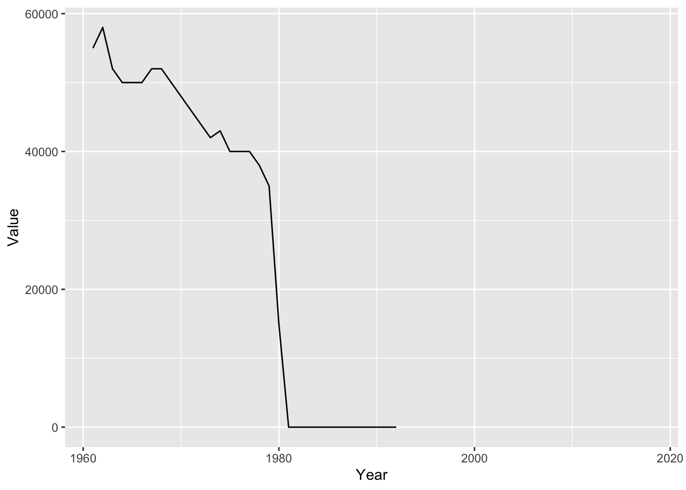

Using the Table function, I found that the data for Iran stopped being available after 1994.

Code

(table(pig_analysis$`Flag Description`,pig_analysis$Year))

                    
                     1961 1962 1963 1964 1965 1966 1967 1968 1969 1970 1971
  Data not available    0    0    0    0    0    0    0    0    0    0    0
  FAO estimate          0    0    0    0    0    0    0    0    1    1    1
  Official data         1    1    1    1    1    1    1    1    0    0    0
                    
                     1972 1973 1974 1975 1976 1977 1978 1979 1980 1981 1990
  Data not available    0    0    0    0    0    0    0    0    0    0    0
  FAO estimate          1    0    0    1    1    1    1    1    1    1    0
  Official data         0    1    1    0    0    0    0    0    0    0    1
                    
                     1991 1992 1993 1994 1995 1996 1997 1998 1999 2000 2001
  Data not available    0    0    1    1    1    1    1    1    1    1    1
  FAO estimate          0    0    0    0    0    0    0    0    0    0    0
  Official data         1    1    0    0    0    0    0    0    0    0    0
                    
                     2002 2003 2004 2005 2006 2007 2008 2009 2010 2011 2012
  Data not available    1    1    1    1    1    1    1    1    1    1    1
  FAO estimate          0    0    0    0    0    0    0    0    0    0    0
  Official data         0    0    0    0    0    0    0    0    0    0    0
                    
                     2013 2014 2015 2016 2017 2018
  Data not available    1    1    1    1    1    1
  FAO estimate          0    0    0    0    0    0
  Official data         0    0    0    0    0    0