Challenge 2

challenge_2

Animesh Sengupta

faostat

Author

Animesh Sengupta

Published

August 16, 2022

Code

library(tidyverse)
library(readr)
knitr::opts_chunk$set(echo = TRUE, warning=FALSE, message=FALSE)

Challenge Overview

Today’s challenge is to

read in a data set, and describe the data using both words and any supporting information (e.g., tables, etc)
provide summary statistics for different interesting groups within the data, and interpret those statistics

Read in the Data

Read in one (or more) of the following data sets, available in the posts/_data folder, using the correct R package and command.

FAOstat*.csv ⭐⭐⭐

Code

#! label: Read Data
FAOstat_livestock <- read_csv("../posts/_data/FAOSTAT_livestock.csv")

Add any comments or documentation as needed. More challenging data may require additional code chunks and documentation.

Describe the data

Using a combination of words and results of R commands, can you provide a high level description of the data? Describe as efficiently as possible where/how the data was (likely) gathered, indicate the cases and variables (both the interpretation and any details you deem useful to the reader to fully understand your chosen data).

Code

#Data Dimensions
dim(FAOstat_livestock)

[1] 82116    14

Code

#Data Columns
colnames(FAOstat_livestock)

 [1] "Domain Code"      "Domain"           "Area Code"        "Area"            
 [5] "Element Code"     "Element"          "Item Code"        "Item"            
 [9] "Year Code"        "Year"             "Unit"             "Value"           
[13] "Flag"             "Flag Description"

Code

#Data Preview
head(FAOstat_livestock,3)

# A tibble: 3 × 14
  Domai…¹ Domain Area …² Area  Eleme…³ Element Item …⁴ Item  Year …⁵  Year Unit 
  <chr>   <chr>    <dbl> <chr>   <dbl> <chr>     <dbl> <chr>   <dbl> <dbl> <chr>
1 QA      Live …       2 Afgh…    5111 Stocks     1107 Asses    1961  1961 Head 
2 QA      Live …       2 Afgh…    5111 Stocks     1107 Asses    1962  1962 Head 
3 QA      Live …       2 Afgh…    5111 Stocks     1107 Asses    1963  1963 Head 
# … with 3 more variables: Value <dbl>, Flag <chr>, `Flag Description` <chr>,
#   and abbreviated variable names ¹`Domain Code`, ²`Area Code`,
#   ³`Element Code`, ⁴`Item Code`, ⁵`Year Code`
# ℹ Use `colnames()` to see all variable names

Processed Data for analysis and some information about it

Code

#! label: Isolate data for analysis
FAOstat_livestock_main <- select(FAOstat_livestock,"Area","Item","Year","Unit","Value")
head(FAOstat_livestock_main,5)

# A tibble: 5 × 5
  Area        Item   Year Unit    Value
  <chr>       <chr> <dbl> <chr>   <dbl>
1 Afghanistan Asses  1961 Head  1300000
2 Afghanistan Asses  1962 Head   851850
3 Afghanistan Asses  1963 Head  1001112
4 Afghanistan Asses  1964 Head  1150000
5 Afghanistan Asses  1965 Head  1300000

Code

countries_num<-n_distinct(FAOstat_livestock_main$Area)
year_vector<-unique(FAOstat_livestock_main$Year)
unique(FAOstat_livestock_main$Item)

[1] "Asses"     "Camels"    "Cattle"    "Goats"     "Horses"    "Mules"    
[7] "Sheep"     "Buffaloes" "Pigs"

The data collected for FAO was between 1961 to 2018 for Areas in total.

I am interested in finding the expenditure statistics on livestock for these countries. Lets find out below.

Provide Grouped Summary Statistics

Conduct some exploratory data analysis, using dplyr commands such as group_by(), select(), filter(), and summarise(). Find the central tendency (mean, median, mode) and dispersion (standard deviation, mix/max/quantile) for different subgroups within the data set.

Code

ct_analysis <- FAOstat_livestock_main %>%
                group_by(Area,Item)%>%
                summarise(mean_val=mean(Value,na.rm = TRUE),
                          median_val=median(Value,na.rm = TRUE),
                          .groups = 'drop')
dim(ct_analysis)

[1] 1566    4

Code

colnames(ct_analysis)

[1] "Area"       "Item"       "mean_val"   "median_val"

##Item wise by analysis

Code

ct_item_group <- ct_analysis %>%
  group_by(Item)%>%
  summarise(mean_val=mean(mean_val,na.rm = TRUE))%>%
  arrange(desc(mean_val))

head(ct_item_group,5)

# A tibble: 5 × 2
  Item       mean_val
  <chr>         <dbl>
1 Cattle    21058163.
2 Sheep     20137879.
3 Pigs      14207291.
4 Goats     10801180.
5 Buffaloes  8583673.

As per the data , Cattle generates the most value for any country , with the mean value being 2.1058163^{7}. We can speculatively attribute this high value to cattle due to its important role in society. For example, a cattle generates value not only be meat consumption but also dairy production. On the other hand, the Mule with lowest mean value of 4.4022093^{5}, has lesser societal value.

##Area wise analysis

Code

ct_area_group <- ct_analysis %>%
  group_by(Area)%>%
  summarise(mean_val=mean(mean_val,na.rm = TRUE))%>%
  arrange(desc(mean_val))

head(ct_area_group,15)

# A tibble: 15 × 2
   Area                        mean_val
   <chr>                          <dbl>
 1 World                     449961866.
 2 Asia                      190587493.
 3 Americas                   95795716.
 4 Eastern Asia               80092992.
 5 Southern Asia              78704652.
 6 Africa                     78159910.
 7 China, mainland            73083831.
 8 Europe                     71745016.
 9 South America              56288859.
10 India                      48618161.
11 USSR                       36287113.
12 Australia and New Zealand  36010992.
13 Eastern Europe             34383679.
14 Oceania                    31265613.
15 Northern America           29793900.

Among the countries, Mainland China and India are the biggest mean producer of livestock value.

##Time wise analysis of largest producer for most valuable livestock

Code

ct_time_series <- FAOstat_livestock_main %>%
  filter(Item == 'Cattle' & Area == 'China, mainland')%>%
  group_by(Year)%>%
  summarise(mean_val=mean(Value,na.rm = TRUE))%>%
  arrange(Year)

ggplot(data = ct_time_series, aes(x = Year, y = mean_val)) +
  geom_point()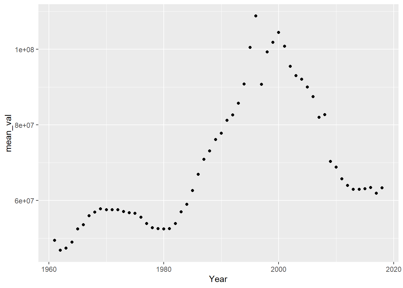

As per the time chart plot, the cattle production started to increase substantially during the late 1900s and saw a peak during early 2000. Since then cattle production has a seen a downfall, probably attributing to advent of technology

Explain and Interpret

For my analysis I chose the subgroup of Area, Item, Time and Value from the FAO Livestock dataset. The reason for choosing such a group of features was because of its high meaningfulness. This would also allow me to conduct Area wise, Item wise and time series Analysis. Conclusion to my analysis would be that Cattle is the MVP while China is the largest producer of livestock.