Challenge 2 Will Munson

Code

library(tidyverse)

knitr::opts_chunk$set(echo = TRUE, warning=FALSE, message=FALSE)

Challenge Overview

Today’s challenge is to

1. read in a data set, and describe the data using both words and any supporting information (e.g., tables, etc)
2. provide summary statistics for different interesting groups within the data, and interpret those statistics

Read in the Data

Read in one (or more) of the following data sets, available in the posts/_data folder, using the correct R package and command.

• railroad*.csv or StateCounty2012.xlsx ⭐
• FAOstat*.csv ⭐⭐⭐
• hotel_bookings ⭐⭐⭐⭐

Code

FAOstat <- read_csv("_data/FAOSTAT_livestock.csv")

Add any comments or documentation as needed. More challenging data may require additional code chunks and documentation.

Describe the data

Using a combination of words and results of R commands, can you provide a high level description of the data? Describe as efficiently as possible where/how the data was (likely) gathered, indicate the cases and variables (both the interpretation and any details you deem useful to the reader to fully understand your chosen data).

So, essentially, this data is interpreting the value of livestock around the world. The values are either official or unofficial data, or FAO estimates. 

The data has a total of over 82k slots. Value is the only quantitative variable. Each set of data was recorded between the years of 1961 and 2018. 

Code

summary(FAOstat)

 Domain Code           Domain            Area Code          Area          
 Length:82116       Length:82116       Min.   :   1.0   Length:82116      
 Class :character   Class :character   1st Qu.:  73.0   Class :character  
 Mode  :character   Mode  :character   Median : 146.0   Mode  :character  
                                       Mean   : 912.7                     
                                       3rd Qu.: 221.0                     
                                       Max.   :5504.0                     
                                                                          
  Element Code    Element            Item Code        Item          
 Min.   :5111   Length:82116       Min.   : 866   Length:82116      
 1st Qu.:5111   Class :character   1st Qu.: 976   Class :character  
 Median :5111   Mode  :character   Median :1034   Mode  :character  
 Mean   :5111                      Mean   :1018                     
 3rd Qu.:5111                      3rd Qu.:1096                     
 Max.   :5111                      Max.   :1126                     
                                                                    
   Year Code         Year          Unit               Value          
 Min.   :1961   Min.   :1961   Length:82116       Min.   :0.000e+00  
 1st Qu.:1976   1st Qu.:1976   Class :character   1st Qu.:1.250e+04  
 Median :1991   Median :1991   Mode  :character   Median :2.247e+05  
 Mean   :1990   Mean   :1990                      Mean   :1.163e+07  
 3rd Qu.:2005   3rd Qu.:2005                      3rd Qu.:2.377e+06  
 Max.   :2018   Max.   :2018                      Max.   :1.490e+09  
                                                  NA's   :1301       
     Flag           Flag Description  
 Length:82116       Length:82116      
 Class :character   Class :character  
 Mode  :character   Mode  :character  
                                      
                                      
                                      
                                      

Provide Grouped Summary Statistics

Conduct some exploratory data analysis, using dplyr commands such as group_by(), select(), filter(), and summarise(). Find the central tendency (mean, median, mode) and dispersion (standard deviation, mix/max/quantile) for different subgroups within the data set.

Code

FAOstat %>%
  group_by(Year) %>%
  filter(Item == 'Sheep' & `Flag Description` == 'Official data') %>%
  summarize(mean = mean(Value, na.rm = TRUE), sd = sd(Value, na.rm = TRUE))

# A tibble: 58 × 3
    Year     mean        sd
   <dbl>    <dbl>     <dbl>
 1  1961 9172935. 22937872.
 2  1962 8667943. 23653127.
 3  1963 8787122. 24057267.
 4  1964 8612111. 23824573.
 5  1965 8492538. 23745915.
 6  1966 9094943. 23326897.
 7  1967 7984239. 22894441.
 8  1968 8688126. 24101623.
 9  1969 8518124. 24300499.
10  1970 7955016. 24019630.
# … with 48 more rows
# ℹ Use `print(n = ...)` to see more rows

I added a chart here to get a better understanding of how the mean official data has changed overtime. Just having the numbers here isn't as helpful as having a chart.

Code

FAO <- FAOstat %>%
  group_by(Year) %>%
  filter(Item == 'Sheep' & `Flag Description` == 'Official data') %>%
  summarize(mean = mean(Value, na.rm = TRUE), sd = sd(Value, na.rm = TRUE))

plot(x = FAO$Year, y = FAO$mean)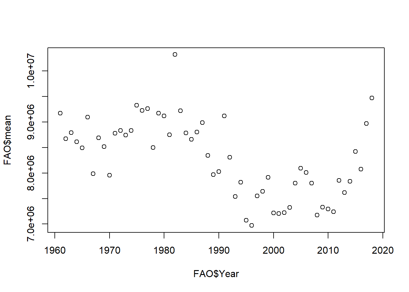

Explain and Interpret

Be sure to explain why you choose a specific group. Comment on the interpretation of any interesting differences between groups that you uncover. This section can be integrated with the exploratory data analysis, just be sure it is included.

This specific group I chose involved sheep and official data. Since the value changes every year, I chose to take the average value and standard deviation of sheep for each year. What appears to be happening here is the mean is the average value of sheep appears to be relatively stagnant between the years 2000 and 2010. After 2010, the official data shows a major surplus in the value of sheep.