library(dplyr)library(ggplot2)animal_weight <-read.csv("_data/animal_weight.csv")#So this dataset covers the (I'm assuming average) weight of different farm animals/farm-adjacent animals in difference areas of the world. For instance, some columns are the usual "cattle, chickens, swine, etc.", but others include camels, llamas, and buffalo. #The geographic areas the data was pulled from are: Indian Subcontinent, Eastern Europe, Africa, Oceania, Western Europe, Latin America, Asia, Middle East, and Northern America.
#NOTE: The data does not specify the unit of weight, but given that Buffalo weigh way more than 380lbs I'm assuming that the measurements are in kilos/kg.
#In order to make the tidying process easier I'm going to start by renaming the columns. As they are, the names aren't super easy to code, so lets fix that!animal_weightr1 <- animal_weight %>%rename(ipcc_area ='IPCC.Area', cattle_dairy ='Cattle...dairy', cattle_nondairy ='Cattle...non.dairy', special_buffaloes ='Buffaloes', swine_market ='Swine...market', swine_breeding ='Swine...breeding', chicken_br ='Chicken...Broilers', chicken_lyr ='Chicken...Layers', ducks ='Ducks', turkeys ='Turkeys', standard_sheep ='Sheep', standard_goats ='Goats', equine_horses ='Horses', equine_asses ='Asses', equine_mules ='Mules', special_camels ='Camels', special_llamas ='Llamas')view(animal_weightr1)
#Now that everything has been renamed, I'm going to start re-grouping columns using the pivot_longer() function. I tried to streamline this but I couldn't get it to work so I did all of it individually.animal_weightr2 <- animal_weightr1 %>%pivot_longer(cols =c(contains("cattle")), names_to ="all_cattle", values_to ="Cattle Weight kg") %>%arrange(all_cattle)animal_weightr3 <- animal_weightr2 %>%pivot_longer(cols =c(contains("equine")), names_to ="all_equine", values_to ="Equine Weight kg") %>%arrange(all_equine)animal_weightr4 <- animal_weightr3 %>%pivot_longer(cols =c(contains("special")), names_to ="specialty_animals", values_to ="Specialized Weight kg") %>%arrange(specialty_animals)animal_weightr5 <- animal_weightr4 %>%pivot_longer(cols =c(contains("standard")), names_to ="standard_farm", values_to ="Standard Weight kg") %>%arrange(standard_farm)animal_weightr6 <- animal_weightr5 %>%pivot_longer(cols =c(contains("swine")), names_to ="all_swine", values_to ="Pigs Weight kg") %>%arrange(all_swine)animal_weightr7 <- animal_weightr6 %>%pivot_longer(cols =c(contains("chicken")), names_to ="all_chickens", values_to ="Chickens Weight kg") %>%arrange(all_chickens)animal_weightr8 <- animal_weightr7 %>%pivot_longer(cols =c("ducks","turkeys"), names_to ="farm_birds", values_to ="Farm Birds Weight kg") %>%arrange(farm_birds)view(animal_weightr8)
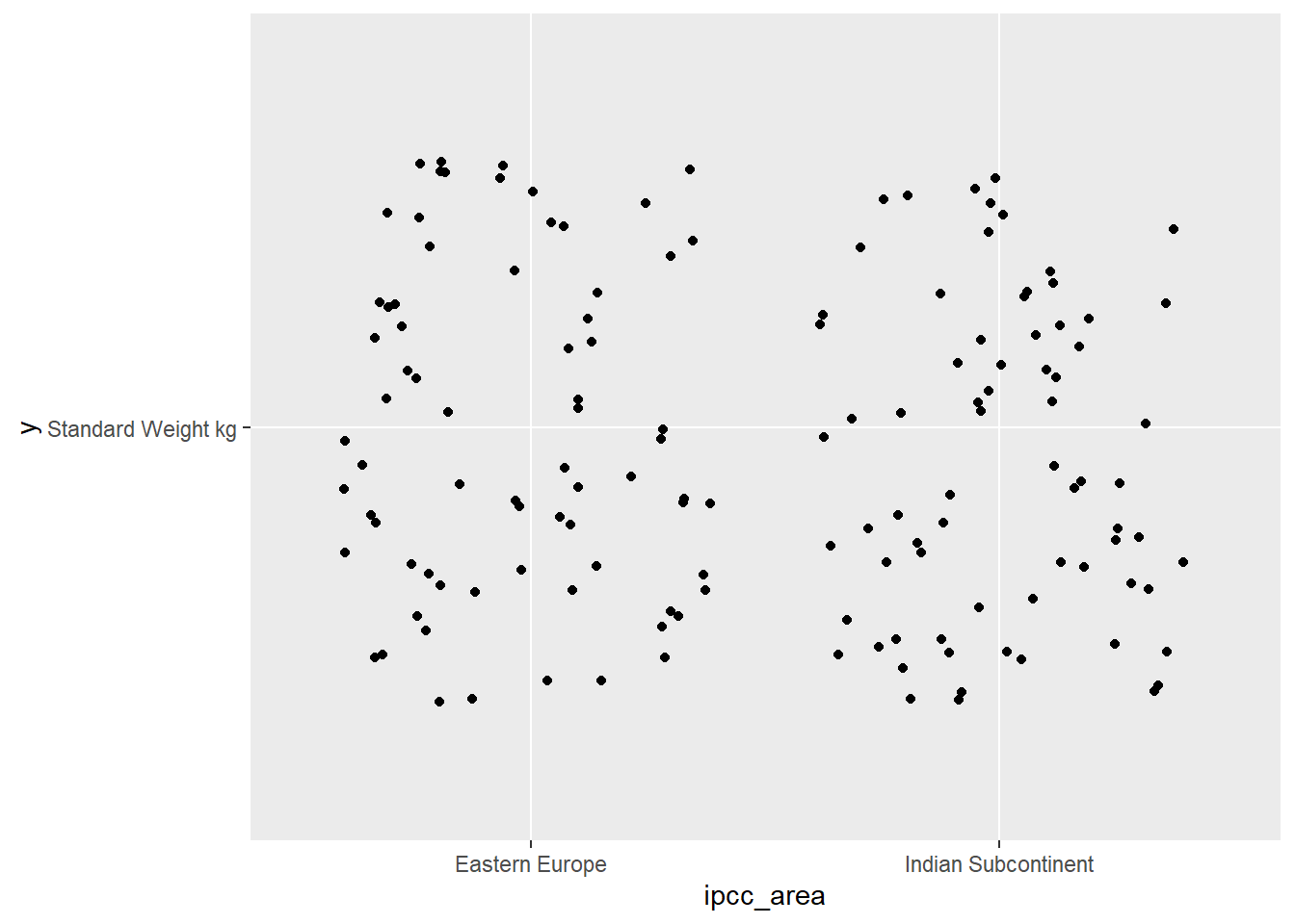
#Now that all the columns are grouped together accordingly, I'm going to look more specifically at animals in a specific geographic area. I chose to look at the weight of sheep in Eastern Europe.animal_weightr8 %>%select(ipcc_area, standard_farm, `Standard Weight kg`) %>%filter(ipcc_area =="Eastern Europe", standard_farm =="standard_goats") %>%view()
#Since the average weight (kg) for goats in Eastern Europe is 38.5kg, I'm going to add in a different geographical area for the purpose of visualsanimal_weight_final <- animal_weightr8 %>%select(ipcc_area, standard_farm, `Standard Weight kg`) %>%filter(ipcc_area ==c("Eastern Europe","Indian Subcontinent"), standard_farm =="standard_goats") %>%view()