Challenge 5

Introduction to Visualization

Code

library(tidyverse)
library(ggplot2)

knitr::opts_chunk$set(echo = TRUE, warning=FALSE, message=FALSE)

Read in data

Code

AB_NYC_2019 <- read_csv("_data/AB_NYC_2019.csv") %>%
  select(!c("id", "host_id", "neighbourhood", "latitude", "longitude", "minimum_nights", "last_review"))
AB_NYC_2019

Briefly describe the data

Code

dim(AB_NYC_2019)

[1] 48895     9

Code

summary(AB_NYC_2019)

     name            host_name         neighbourhood_group  room_type        
 Length:48895       Length:48895       Length:48895        Length:48895      
 Class :character   Class :character   Class :character    Class :character  
 Mode  :character   Mode  :character   Mode  :character    Mode  :character  
                                                                             
                                                                             
                                                                             
                                                                             
     price         number_of_reviews reviews_per_month
 Min.   :    0.0   Min.   :  0.00    Min.   : 0.010   
 1st Qu.:   69.0   1st Qu.:  1.00    1st Qu.: 0.190   
 Median :  106.0   Median :  5.00    Median : 0.720   
 Mean   :  152.7   Mean   : 23.27    Mean   : 1.373   
 3rd Qu.:  175.0   3rd Qu.: 24.00    3rd Qu.: 2.020   
 Max.   :10000.0   Max.   :629.00    Max.   :58.500   
                                     NA's   :10052    
 calculated_host_listings_count availability_365
 Min.   :  1.000                Min.   :  0.0   
 1st Qu.:  1.000                1st Qu.:  0.0   
 Median :  1.000                Median : 45.0   
 Mean   :  7.144                Mean   :112.8   
 3rd Qu.:  2.000                3rd Qu.:227.0   
 Max.   :327.000                Max.   :365.0   
                                                

Tidy Data (as needed)

Code

AB_NYC_2019 <- replace_na(AB_NYC_2019, list(reviews_per_month = 0))
AB_NYC_2019

Code

dim(AB_NYC_2019)

[1] 48895     9

Code

summary(AB_NYC_2019)

     name            host_name         neighbourhood_group  room_type        
 Length:48895       Length:48895       Length:48895        Length:48895      
 Class :character   Class :character   Class :character    Class :character  
 Mode  :character   Mode  :character   Mode  :character    Mode  :character  
                                                                             
                                                                             
                                                                             
     price         number_of_reviews reviews_per_month
 Min.   :    0.0   Min.   :  0.00    Min.   : 0.000   
 1st Qu.:   69.0   1st Qu.:  1.00    1st Qu.: 0.040   
 Median :  106.0   Median :  5.00    Median : 0.370   
 Mean   :  152.7   Mean   : 23.27    Mean   : 1.091   
 3rd Qu.:  175.0   3rd Qu.: 24.00    3rd Qu.: 1.580   
 Max.   :10000.0   Max.   :629.00    Max.   :58.500   
 calculated_host_listings_count availability_365
 Min.   :  1.000                Min.   :  0.0   
 1st Qu.:  1.000                1st Qu.:  0.0   
 Median :  1.000                Median : 45.0   
 Mean   :  7.144                Mean   :112.8   
 3rd Qu.:  2.000                3rd Qu.:227.0   
 Max.   :327.000                Max.   :365.0   

Univariate Visualizations

Code

ggplot(AB_NYC_2019, aes(price)) + 
  geom_histogram(fill = "blue") + 
  xlim(0,1700) +
  labs(title = "Price of the room", x = "Price", y = "Frequency") + 
  theme_bw()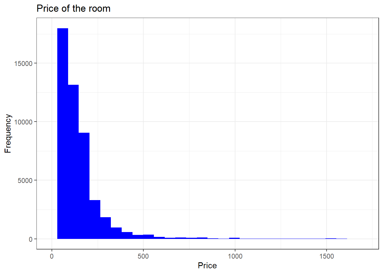

Code

ggplot(AB_NYC_2019, aes(number_of_reviews)) + 
  geom_histogram(fill = "lightgreen") + 
  xlim(0,400) +
  labs(title = "No of reviews", x = "Reviews", y = "Frequency") + 
  theme_bw()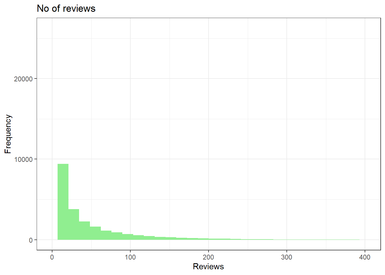

Code

ggplot(AB_NYC_2019, aes(reviews_per_month)) + 
  geom_histogram(fill = "red") + 
  xlim(0,15) +
  labs(title = "Reviews in a month", x = "Monthly reviews", y = "Frequency") + 
  theme_bw()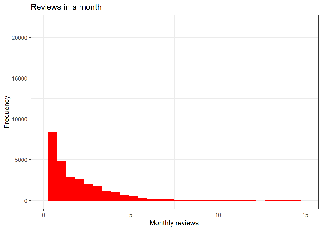

Code

ggplot(AB_NYC_2019, aes(availability_365)) + 
  geom_histogram(fill = "orange") + 
  xlim(0,370) +
  labs(title = "Availability of the room", x = "Availability", y = "Frequency") + 
  theme_bw()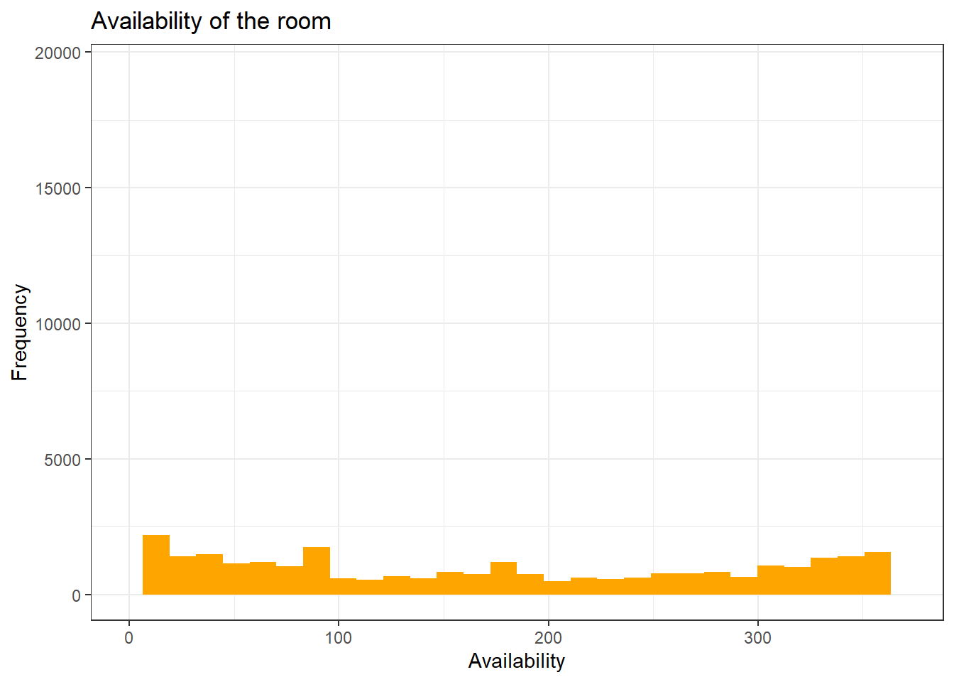

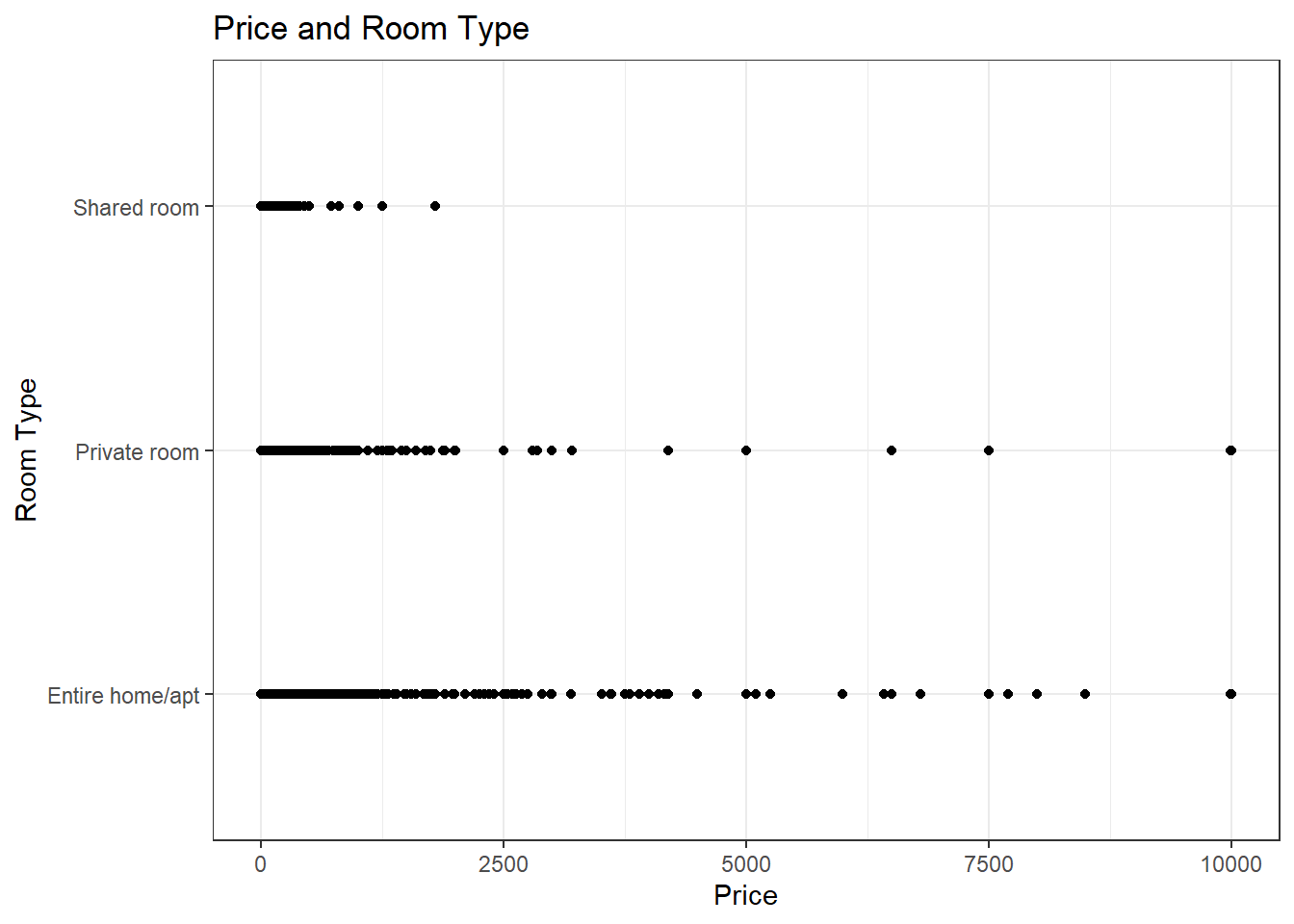
Bivariate Visualization(s)

Code

ggplot(AB_NYC_2019, aes(price, room_type)) + 
  geom_point() + 
  labs(title = "Price and Room Type", x = "Price", y = "Room Type") + 
  theme_bw()