Generated by summarytools 1.0.1 (R version 4.2.1) 2022-08-28
Describe the data and Tidy
After reading in the data I can tell I am dealing with NYC Air BnB data from 2019. To Tidy the data, I removed the id columns and rows with a value of 0 in them for number_of_reviews. The reason for this is that number_of_reivews will be a focal point of the analysis for this dataset. I want to compare number of reviews with other variables to see if reviews have any effect whether it is the independent or dependent variable. By looking at the summary table I could also investigate the number of reviews for each neighborhood_group and neighborhood.
Univariate Visualizations
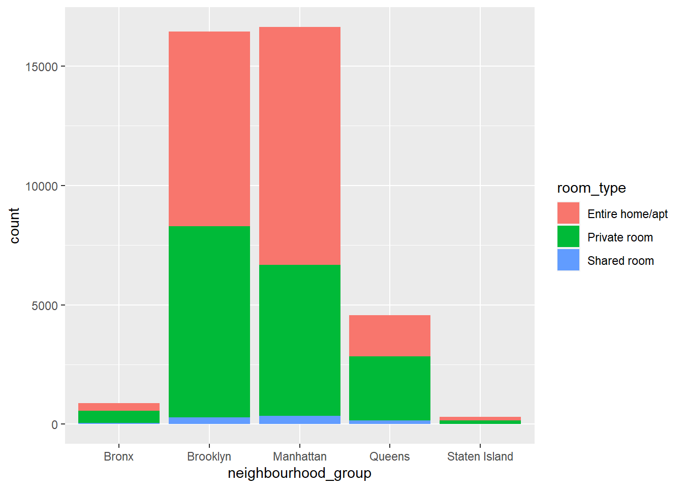
ggplot(data = AB) +geom_bar(mapping =aes(x = neighbourhood_group, fill = room_type))
AB_n <- AB %>%group_by(neighbourhood_group) %>%summarise(number_of_reviews =sum(number_of_reviews))AB_n
Here I created a Bar chart that counts the number of instances in a neighborhood group. I used the fill function to see which neighborhoods offer different types of rooms. Based on the results I can see that Brooklyn and Manhattan take up majority of the Air Bnbs in NYC. Also, within those two neighborhoods I can see that most of the Air BnBs are either a entire home/apt or a Private room. The Bronx and Staten Island do not offer any shared rooms.
Bivariate Visualization(s)
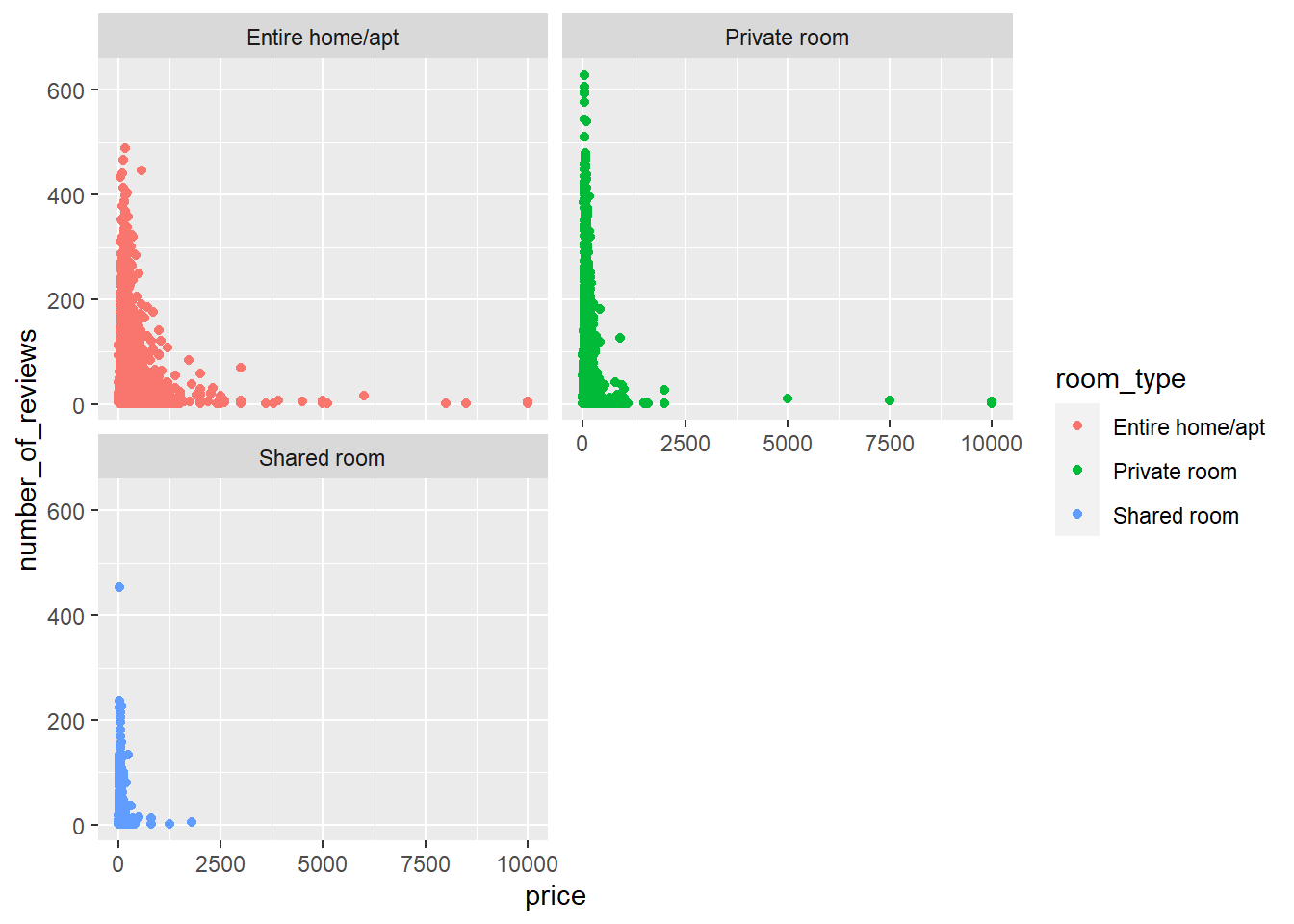
ggplot(data = AB) +geom_point(mapping =aes(x = price, y = number_of_reviews, color =room_type))+facet_wrap(~ room_type, nrow =2)
Here I created subplots that each display price ad the X axis and each room_type as the Y axis. Based on the results I can see that around the price of 500, the amount of reviews starts to decline for all room types. One problem with these graphs is that they are out of scop making it hard to visualize what is going on.
Source Code
---title: "Challenge 5"author: "Nayan Jani"description: "Introduction to Visualization"date: "08/22/2022"format: html: df-print: paged toc: true code-copy: true code-tools: truecategories: - challenge_5 - railroads - cereal - air_bnb - pathogen_cost - australian_marriage - public_schools - usa_hh---```{r}#| label: setup#| warning: false#| message: falselibrary(tidyverse)library(ggplot2)library(summarytools)knitr::opts_chunk$set(echo =TRUE, warning=FALSE, message=FALSE)```## Read in data```{r}AB <-read_csv("_data/AB_NYC_2019.csv", col_names =c("del", "name", "del", "host_name","neighbourhood_group", "neighbourhood", "latitude", "longitude", "room_type", "price", "minimum_nights", "number_of_reviews", "last_review", "reviews_per_month", "calculated_host_listings_count", "availability_365" ), skip=1) %>%select(!starts_with("del")) %>%drop_na(reviews_per_month)ABprint(dfSummary(AB, varnumbers =FALSE,plain.ascii =FALSE, style ="grid", graph.magnif =0.70, valid.col =FALSE),method ='render',table.classes ='table-condensed')```### Describe the data and TidyAfter reading in the data I can tell I am dealing with NYC Air BnB data from 2019. To Tidy the data, I removed the id columns and rows with a value of 0 in them for number_of_reviews. The reason for this is that number_of_reivews will be a focal point of the analysis for this dataset. I want to compare number of reviews with other variables to see if reviews have any effect whether it is the independent or dependent variable. By looking at the summary table I could also investigate the number of reviews for each neighborhood_group and neighborhood.## Univariate Visualizations```{r}ggplot(data = AB) +geom_bar(mapping =aes(x = neighbourhood_group, fill = room_type))AB_n <- AB %>%group_by(neighbourhood_group) %>%summarise(number_of_reviews =sum(number_of_reviews))AB_n```Here I created a Bar chart that counts the number of instances in a neighborhood group. I used the fill function to see which neighborhoods offer different types of rooms. Based on the results I can see that Brooklyn and Manhattan take up majority of the Air Bnbs in NYC. Also, within those two neighborhoods I can see that most of the Air BnBs are either a entire home/apt or a Private room. The Bronx and Staten Island do not offer any shared rooms.## Bivariate Visualization(s)```{r}ggplot(data = AB) +geom_point(mapping =aes(x = price, y = number_of_reviews, color =room_type))+facet_wrap(~ room_type, nrow =2)```Here I created subplots that each display price ad the X axis and each room_type as the Y axis. Based on the results I can see that around the price of 500, the amount of reviews starts to decline for all room types. One problem with these graphs is that they are out of scop making it hard to visualize what is going on.