Eventhough the file name says the data contains 15 pathogens, the actual dataset has 27 rows which means there are certain rows to be dropped. There are 3 columns/variable; the name of the pathogen, number of cases and the total cost caused by the pathogen in the year.
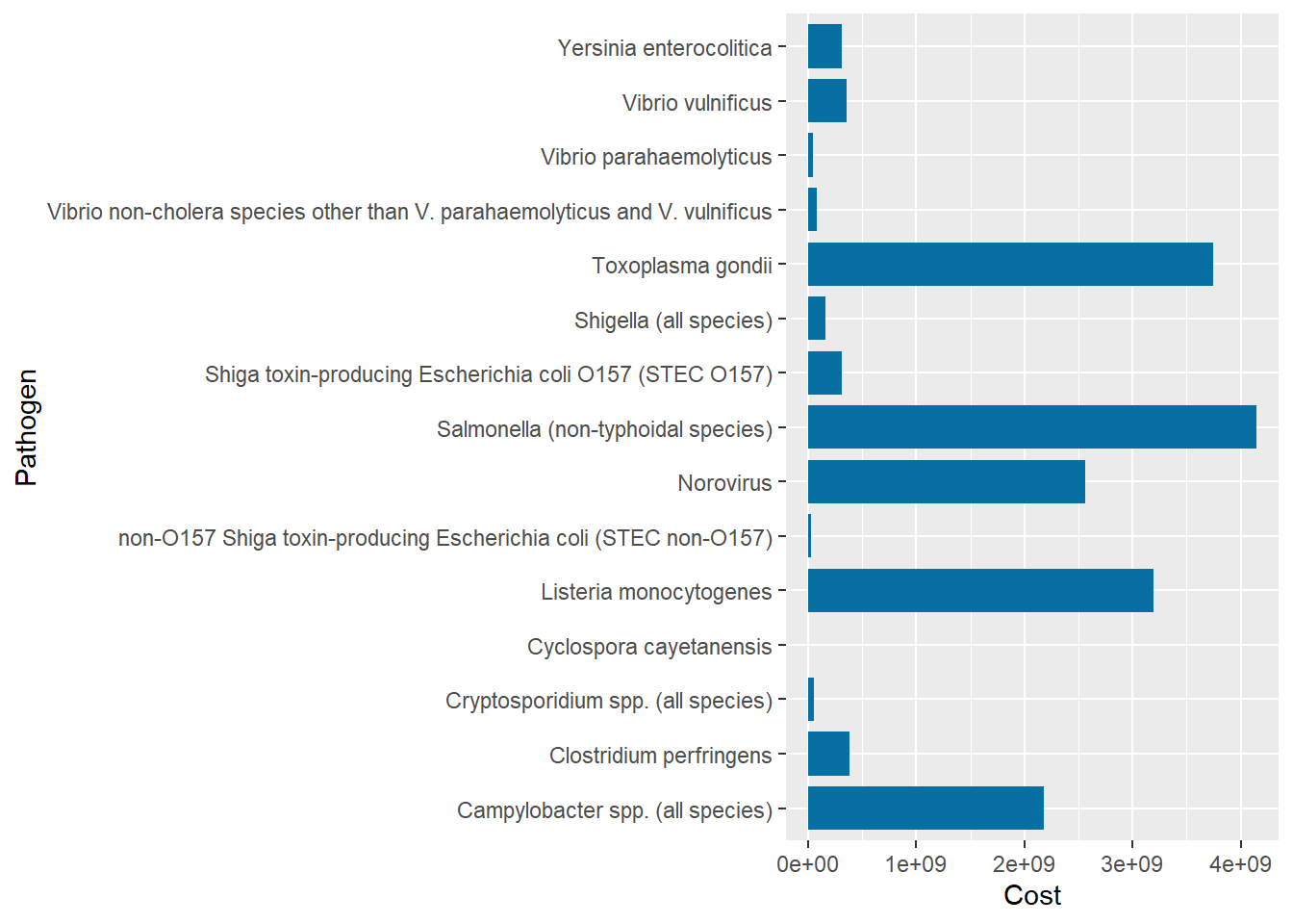
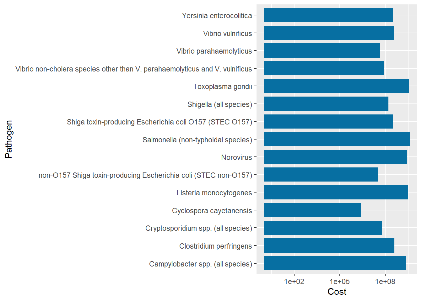
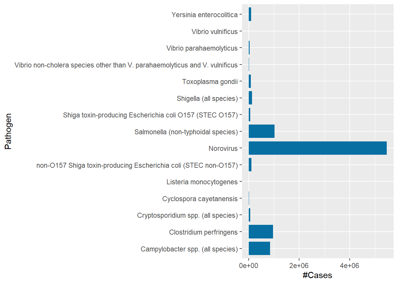
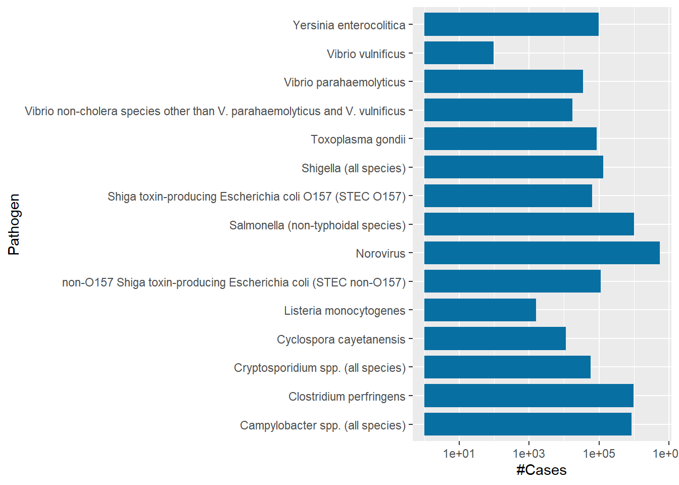
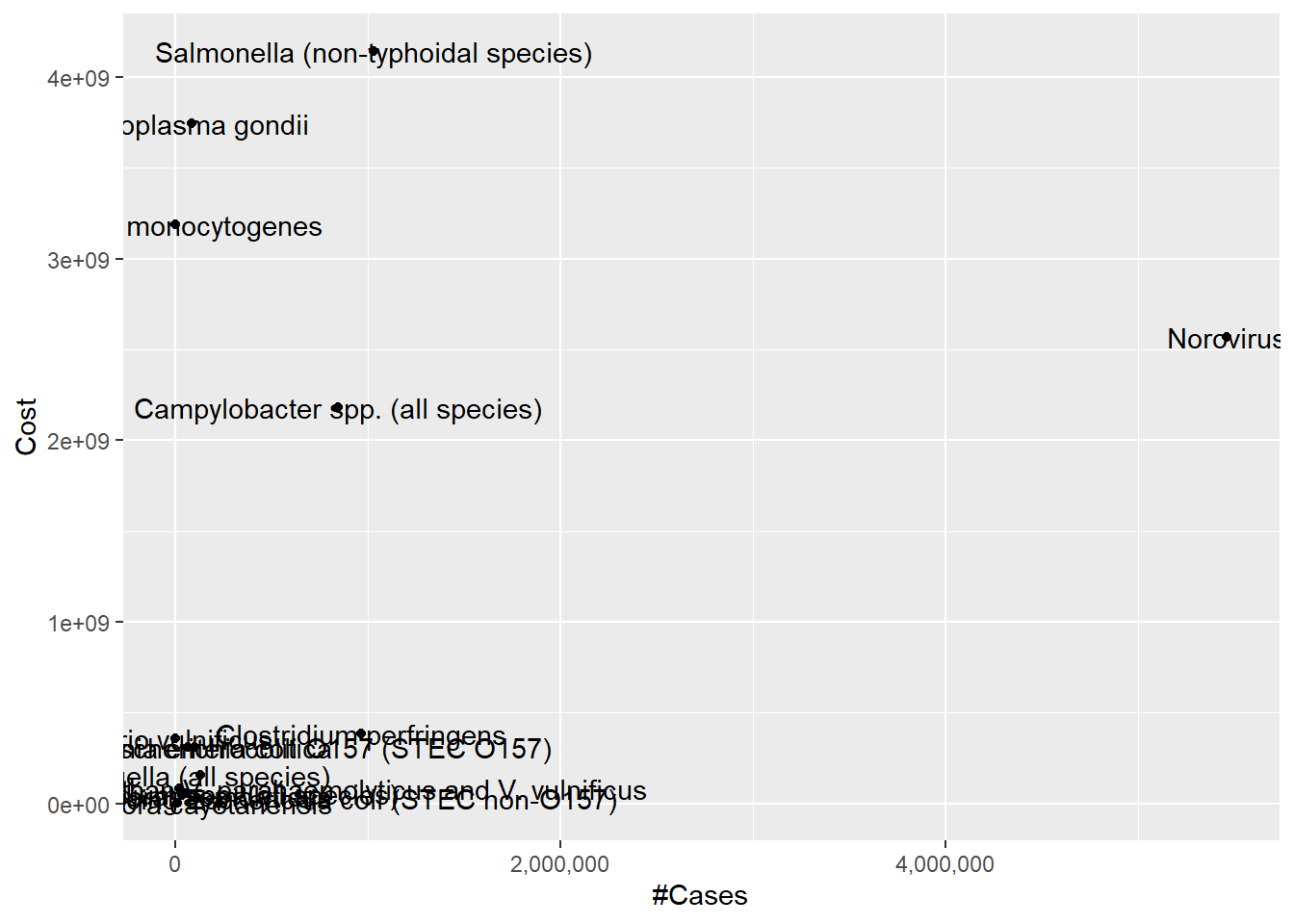
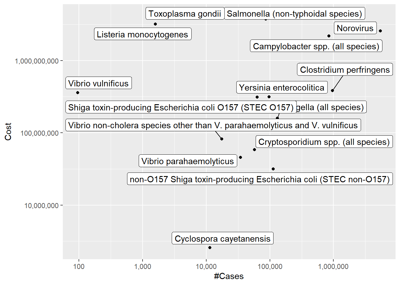
Vibrio vulnificus had the least number of cases, just 96 cases, in 2018 while Norovirus came first with 5461731 reported cases. Cyclospora Cayetanensis cost the least in total ($2571518) and Salmonella (non-typhoidal species) cost the most that totalled to 4142179161.
summary(pathogen)
   Pathogen             #Cases             Cost
 Length:15          Min.   :     96   Min.   :2.572e+06
 Class :character   1st Qu.:  26114   1st Qu.:7.007e+07
 Mode  :character   Median :  86686   Median :3.133e+08
                    Mean   : 594314   Mean   :1.171e+09
                    3rd Qu.: 488139   3rd Qu.:2.374e+09
                    Max.   :5461731   Max.   :4.142e+09
---title: "Challenge 5"author: "Jerin Jacob"description: "Introduction to Visualization"date: "08/22/2022"format: html: toc: true code-copy: true code-tools: truecategories: - challenge_5 - pathogen_cost---I am working on the Cost of Pathogens dataset for the year of 2018.```{r}#| label: setup#| warning: false#| message: falselibrary(tidyverse)library(ggplot2)library(readxl)library(dplyr)library(stringr)library(shadowtext)library(scales)knitr::opts_chunk$set(echo =TRUE, warning=FALSE, message=FALSE)```## Read in dataEventhough the file name says the data contains 15 pathogens, the actual dataset has 27 rows which means there are certain rows to be dropped. There are 3 columns/variable; the name of the pathogen, number of cases and the total cost caused by the pathogen in the year.```{r}pathogen <-read_excel("_data/Total_cost_for_top_15_pathogens_2018.xlsx", skip =5, col_names =c("Pathogen", "#Cases", "Cost"), n_max =15)#options(scipen=999)#head(pathogen)dim(pathogen)#pathogen```### Briefly describe the dataVibrio vulnificus had the least number of cases, just 96 cases, in 2018 while Norovirus came first with 5461731 reported cases. Cyclospora Cayetanensis cost the least in total ($2571518) and Salmonella (non-typhoidal species) cost the most that totalled to 4142179161.```{r}summary(pathogen)pathogen[which.min(pathogen$`#Cases`),]pathogen[which.max(pathogen$`#Cases`),]pathogen[which.min(pathogen$Cost),]pathogen[which.max(pathogen$Cost),]```## Tidy Data (as needed)The data has been mutated by adding a new variable called Average Cost per cases so that we can study how the cost per cases of each pathogen varies. ```{r}pathogen %>%mutate(Avg_Cost_per_case = Cost/`#Cases`)head(pathogen)```## Univariate Visualizations```{r}BLUE <-"#076fa2"ggplot(pathogen) +geom_col(aes(Cost, Pathogen), fill = BLUE, width = .8)ggplot(pathogen) +geom_col(aes(Cost, Pathogen), fill = BLUE, width = .8) +scale_x_continuous(trans ="log10")ggplot(pathogen) +geom_col(aes(`#Cases`, Pathogen), fill = BLUE, width = .8)ggplot(pathogen) +geom_col(aes(`#Cases`, Pathogen), fill = BLUE, width = .8) +scale_x_continuous(trans ="log10")```## Bivariate Visualization(s)```{r}ggplot(pathogen, aes(x=`#Cases`, y=Cost, label=Pathogen)) +geom_point() +scale_x_continuous(labels = scales::comma)+geom_text()ggplot(pathogen, aes(x=`#Cases`, y=Cost, label=Pathogen)) +geom_point()+scale_x_continuous(trans ="log10", labels = scales::comma)+scale_y_continuous(trans ="log10", labels = scales::comma)+ ggrepel::geom_label_repel()```