Challenge 6 - Adithya Parupudi

Visualizing Time and Relationships

library(tidyverse)
library(ggplot2)
library(summarytools)
library(readxl)
library(lubridate)

knitr::opts_chunk$set(echo = TRUE, warning=FALSE, message=FALSE)

We will be reading the debt excel sheet

debt <- read_excel('_data/debt_in_trillions.xlsx')
debt

# A tibble: 74 × 8
   `Year and Quarter` Mortgage HE Revolvin…¹ Auto …² Credi…³ Stude…⁴ Other Total
   <chr>                 <dbl>         <dbl>   <dbl>   <dbl>   <dbl> <dbl> <dbl>
 1 03:Q1                  4.94         0.242   0.641   0.688   0.241 0.478  7.23
 2 03:Q2                  5.08         0.26    0.622   0.693   0.243 0.486  7.38
 3 03:Q3                  5.18         0.269   0.684   0.693   0.249 0.477  7.56
 4 03:Q4                  5.66         0.302   0.704   0.698   0.253 0.449  8.07
 5 04:Q1                  5.84         0.328   0.72    0.695   0.260 0.446  8.29
 6 04:Q2                  5.97         0.367   0.743   0.697   0.263 0.423  8.46
 7 04:Q3                  6.21         0.426   0.751   0.706   0.33  0.41   8.83
 8 04:Q4                  6.36         0.468   0.728   0.717   0.346 0.423  9.04
 9 05:Q1                  6.51         0.502   0.725   0.71    0.364 0.394  9.21
10 05:Q2                  6.70         0.528   0.774   0.717   0.374 0.402  9.49
# … with 64 more rows, and abbreviated variable names ¹​`HE Revolving`,
#   ²​`Auto Loan`, ³​`Credit Card`, ⁴​`Student Loan`
# ℹ Use `print(n = ...)` to see more rows

Briefly describe the data

debt_new <- debt %>%
  mutate(date = parse_date_time(`Year and Quarter`, orders="yq"))
debt_new

# A tibble: 74 × 9
   `Year and Quarter` Mortgage HE Revolvin…¹ Auto …² Credi…³ Stude…⁴ Other Total
   <chr>                 <dbl>         <dbl>   <dbl>   <dbl>   <dbl> <dbl> <dbl>
 1 03:Q1                  4.94         0.242   0.641   0.688   0.241 0.478  7.23
 2 03:Q2                  5.08         0.26    0.622   0.693   0.243 0.486  7.38
 3 03:Q3                  5.18         0.269   0.684   0.693   0.249 0.477  7.56
 4 03:Q4                  5.66         0.302   0.704   0.698   0.253 0.449  8.07
 5 04:Q1                  5.84         0.328   0.72    0.695   0.260 0.446  8.29
 6 04:Q2                  5.97         0.367   0.743   0.697   0.263 0.423  8.46
 7 04:Q3                  6.21         0.426   0.751   0.706   0.33  0.41   8.83
 8 04:Q4                  6.36         0.468   0.728   0.717   0.346 0.423  9.04
 9 05:Q1                  6.51         0.502   0.725   0.71    0.364 0.394  9.21
10 05:Q2                  6.70         0.528   0.774   0.717   0.374 0.402  9.49
# … with 64 more rows, 1 more variable: date <dttm>, and abbreviated variable
#   names ¹​`HE Revolving`, ²​`Auto Loan`, ³​`Credit Card`, ⁴​`Student Loan`
# ℹ Use `print(n = ...)` to see more rows, and `colnames()` to see all variable names

Time Dependent Visualization

debt_new %>% 
  ggplot(aes(date,Total)) +
  geom_point(size=.5) +
  geom_line()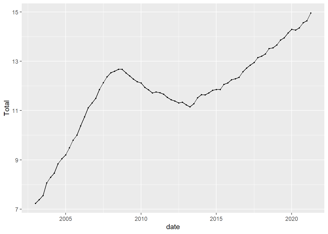 

Visualizing Part-Whole Relationships

Not sure about this part. Have to study on this more.