Code
library(tidyverse)
library(ggplot2)

knitr::opts_chunk$set(echo = TRUE, warning=FALSE, message=FALSE)library(tidyverse)
library(ggplot2)
knitr::opts_chunk$set(echo = TRUE, warning=FALSE, message=FALSE)Read the data about FAO.
fao_egg<-read_csv("_data/FAOSTAT_egg_chicken.csv",show_col_types = FALSE)
fao_egg
# A tibble: 38,170 × 14
Domain Cod…¹ Domain Area …² Area Eleme…³ Element Item …⁴ Item Year …⁵ Year
<chr> <chr> <dbl> <chr> <dbl> <chr> <dbl> <chr> <dbl> <dbl>
1 QL Lives… 2 Afgh… 5313 Laying 1062 Eggs… 1961 1961
2 QL Lives… 2 Afgh… 5410 Yield 1062 Eggs… 1961 1961
3 QL Lives… 2 Afgh… 5510 Produc… 1062 Eggs… 1961 1961
4 QL Lives… 2 Afgh… 5313 Laying 1062 Eggs… 1962 1962
5 QL Lives… 2 Afgh… 5410 Yield 1062 Eggs… 1962 1962
6 QL Lives… 2 Afgh… 5510 Produc… 1062 Eggs… 1962 1962
7 QL Lives… 2 Afgh… 5313 Laying 1062 Eggs… 1963 1963
8 QL Lives… 2 Afgh… 5410 Yield 1062 Eggs… 1963 1963
9 QL Lives… 2 Afgh… 5510 Produc… 1062 Eggs… 1963 1963
10 QL Lives… 2 Afgh… 5313 Laying 1062 Eggs… 1964 1964
# … with 38,160 more rows, 4 more variables: Unit <chr>, Value <dbl>,
# Flag <chr>, `Flag Description` <chr>, and abbreviated variable names
# ¹`Domain Code`, ²`Area Code`, ³`Element Code`, ⁴`Item Code`, ⁵`Year Code`
# ℹ Use `print(n = ...)` to see more rows, and `colnames()` to see all variable namesfao_livestock<-read_csv("_data/FAOSTAT_livestock.csv",show_col_types = FALSE)
fao_livestock# A tibble: 82,116 × 14
Domain Cod…¹ Domain Area …² Area Eleme…³ Element Item …⁴ Item Year …⁵ Year
<chr> <chr> <dbl> <chr> <dbl> <chr> <dbl> <chr> <dbl> <dbl>
1 QA Live … 2 Afgh… 5111 Stocks 1107 Asses 1961 1961
2 QA Live … 2 Afgh… 5111 Stocks 1107 Asses 1962 1962
3 QA Live … 2 Afgh… 5111 Stocks 1107 Asses 1963 1963
4 QA Live … 2 Afgh… 5111 Stocks 1107 Asses 1964 1964
5 QA Live … 2 Afgh… 5111 Stocks 1107 Asses 1965 1965
6 QA Live … 2 Afgh… 5111 Stocks 1107 Asses 1966 1966
7 QA Live … 2 Afgh… 5111 Stocks 1107 Asses 1967 1967
8 QA Live … 2 Afgh… 5111 Stocks 1107 Asses 1968 1968
9 QA Live … 2 Afgh… 5111 Stocks 1107 Asses 1969 1969
10 QA Live … 2 Afgh… 5111 Stocks 1107 Asses 1970 1970
# … with 82,106 more rows, 4 more variables: Unit <chr>, Value <dbl>,
# Flag <chr>, `Flag Description` <chr>, and abbreviated variable names
# ¹`Domain Code`, ²`Area Code`, ³`Element Code`, ⁴`Item Code`, ⁵`Year Code`
# ℹ Use `print(n = ...)` to see more rows, and `colnames()` to see all variable namesfao_cattle<-read_csv("_data/FAOSTAT_cattle_dairy.csv",show_col_types = FALSE)
fao_cattle# A tibble: 36,449 × 14
Domain Cod…¹ Domain Area …² Area Eleme…³ Element Item …⁴ Item Year …⁵ Year
<chr> <chr> <dbl> <chr> <dbl> <chr> <dbl> <chr> <dbl> <dbl>
1 QL Lives… 2 Afgh… 5318 Milk A… 882 Milk… 1961 1961
2 QL Lives… 2 Afgh… 5420 Yield 882 Milk… 1961 1961
3 QL Lives… 2 Afgh… 5510 Produc… 882 Milk… 1961 1961
4 QL Lives… 2 Afgh… 5318 Milk A… 882 Milk… 1962 1962
5 QL Lives… 2 Afgh… 5420 Yield 882 Milk… 1962 1962
6 QL Lives… 2 Afgh… 5510 Produc… 882 Milk… 1962 1962
7 QL Lives… 2 Afgh… 5318 Milk A… 882 Milk… 1963 1963
8 QL Lives… 2 Afgh… 5420 Yield 882 Milk… 1963 1963
9 QL Lives… 2 Afgh… 5510 Produc… 882 Milk… 1963 1963
10 QL Lives… 2 Afgh… 5318 Milk A… 882 Milk… 1964 1964
# … with 36,439 more rows, 4 more variables: Unit <chr>, Value <dbl>,
# Flag <chr>, `Flag Description` <chr>, and abbreviated variable names
# ¹`Domain Code`, ²`Area Code`, ³`Element Code`, ⁴`Item Code`, ⁵`Year Code`
# ℹ Use `print(n = ...)` to see more rows, and `colnames()` to see all variable namesfao_country<-read_csv("_data/FAOSTAT_country_groups.csv",show_col_types = FALSE)
fao_country# A tibble: 1,943 × 7
`Country Group Code` `Country Group` Countr…¹ Country M49 C…² ISO2 …³ ISO3 …⁴
<dbl> <chr> <dbl> <chr> <chr> <chr> <chr>
1 5100 Africa 4 Algeria 012 DZ DZA
2 5100 Africa 7 Angola 024 AO AGO
3 5100 Africa 53 Benin 204 BJ BEN
4 5100 Africa 20 Botswa… 072 BW BWA
5 5100 Africa 233 Burkin… 854 BF BFA
6 5100 Africa 29 Burundi 108 BI BDI
7 5100 Africa 35 Cabo V… 132 CV CPV
8 5100 Africa 32 Camero… 120 CM CMR
9 5100 Africa 37 Centra… 140 CF CAF
10 5100 Africa 39 Chad 148 TD TCD
# … with 1,933 more rows, and abbreviated variable names ¹`Country Code`,
# ²`M49 Code`, ³`ISO2 Code`, ⁴`ISO3 Code`
# ℹ Use `print(n = ...)` to see more rowsIt looks like data about egg, chicken, livestock, and cattle. And country data file is maybe the direction of the interpret the domains, and countries that contained in the each data set. So I would like to join all the data except the country data. To do so, I looked up the column names of data.
colnames(fao_cattle) [1] "Domain Code" "Domain" "Area Code" "Area"
[5] "Element Code" "Element" "Item Code" "Item"
[9] "Year Code" "Year" "Unit" "Value"
[13] "Flag" "Flag Description"colnames(fao_livestock) [1] "Domain Code" "Domain" "Area Code" "Area"
[5] "Element Code" "Element" "Item Code" "Item"
[9] "Year Code" "Year" "Unit" "Value"
[13] "Flag" "Flag Description"colnames(fao_egg) [1] "Domain Code" "Domain" "Area Code" "Area"
[5] "Element Code" "Element" "Item Code" "Item"
[9] "Year Code" "Year" "Unit" "Value"
[13] "Flag" "Flag Description"Fortunately, It all have same column names. So I don’t need to transform data to join them.
First of all, I joined cattle and livestock data.
cat_live<-full_join(fao_cattle, fao_livestock)
cat_live
# A tibble: 118,565 × 14
Domain Cod…¹ Domain Area …² Area Eleme…³ Element Item …⁴ Item Year …⁵ Year
<chr> <chr> <dbl> <chr> <dbl> <chr> <dbl> <chr> <dbl> <dbl>
1 QL Lives… 2 Afgh… 5318 Milk A… 882 Milk… 1961 1961
2 QL Lives… 2 Afgh… 5420 Yield 882 Milk… 1961 1961
3 QL Lives… 2 Afgh… 5510 Produc… 882 Milk… 1961 1961
4 QL Lives… 2 Afgh… 5318 Milk A… 882 Milk… 1962 1962
5 QL Lives… 2 Afgh… 5420 Yield 882 Milk… 1962 1962
6 QL Lives… 2 Afgh… 5510 Produc… 882 Milk… 1962 1962
7 QL Lives… 2 Afgh… 5318 Milk A… 882 Milk… 1963 1963
8 QL Lives… 2 Afgh… 5420 Yield 882 Milk… 1963 1963
9 QL Lives… 2 Afgh… 5510 Produc… 882 Milk… 1963 1963
10 QL Lives… 2 Afgh… 5318 Milk A… 882 Milk… 1964 1964
# … with 118,555 more rows, 4 more variables: Unit <chr>, Value <dbl>,
# Flag <chr>, `Flag Description` <chr>, and abbreviated variable names
# ¹`Domain Code`, ²`Area Code`, ³`Element Code`, ⁴`Item Code`, ⁵`Year Code`
# ℹ Use `print(n = ...)` to see more rows, and `colnames()` to see all variable namesThey were joined successfully. The joined data now have 118,565rows. This is exactly the same as livestock and cattle combined. Then, I joined the egg and chicken data into that data.
tot_fao<-full_join(cat_live, fao_egg)
tot_fao
# A tibble: 156,735 × 14
Domain Cod…¹ Domain Area …² Area Eleme…³ Element Item …⁴ Item Year …⁵ Year
<chr> <chr> <dbl> <chr> <dbl> <chr> <dbl> <chr> <dbl> <dbl>
1 QL Lives… 2 Afgh… 5318 Milk A… 882 Milk… 1961 1961
2 QL Lives… 2 Afgh… 5420 Yield 882 Milk… 1961 1961
3 QL Lives… 2 Afgh… 5510 Produc… 882 Milk… 1961 1961
4 QL Lives… 2 Afgh… 5318 Milk A… 882 Milk… 1962 1962
5 QL Lives… 2 Afgh… 5420 Yield 882 Milk… 1962 1962
6 QL Lives… 2 Afgh… 5510 Produc… 882 Milk… 1962 1962
7 QL Lives… 2 Afgh… 5318 Milk A… 882 Milk… 1963 1963
8 QL Lives… 2 Afgh… 5420 Yield 882 Milk… 1963 1963
9 QL Lives… 2 Afgh… 5510 Produc… 882 Milk… 1963 1963
10 QL Lives… 2 Afgh… 5318 Milk A… 882 Milk… 1964 1964
# … with 156,725 more rows, 4 more variables: Unit <chr>, Value <dbl>,
# Flag <chr>, `Flag Description` <chr>, and abbreviated variable names
# ¹`Domain Code`, ²`Area Code`, ³`Element Code`, ⁴`Item Code`, ⁵`Year Code`
# ℹ Use `print(n = ...)` to see more rows, and `colnames()` to see all variable namesNow, It has 156,735 rows that is exactly same as all the number of data is summed.
I read the data about snl.
snl_seasons<-read_csv("_data/snl_seasons.csv",show_col_types = FALSE)
snl_seasons
# A tibble: 46 × 5
sid year first_epid last_epid n_episodes
<dbl> <dbl> <dbl> <dbl> <dbl>
1 1 1975 19751011 19760731 24
2 2 1976 19760918 19770521 22
3 3 1977 19770924 19780520 20
4 4 1978 19781007 19790526 20
5 5 1979 19791013 19800524 20
6 6 1980 19801115 19810411 13
7 7 1981 19811003 19820522 20
8 8 1982 19820925 19830514 20
9 9 1983 19831008 19840512 19
10 10 1984 19841006 19850413 17
# … with 36 more rows
# ℹ Use `print(n = ...)` to see more rowssnl_casts<-read_csv("_data/snl_casts.csv",show_col_types = FALSE)
snl_casts# A tibble: 614 × 8
aid sid featured first_epid last_epid update…¹ n_epi…² seaso…³
<chr> <dbl> <lgl> <dbl> <dbl> <lgl> <dbl> <dbl>
1 A. Whitney Brown 11 TRUE 19860222 NA FALSE 8 0.444
2 A. Whitney Brown 12 TRUE NA NA FALSE 20 1
3 A. Whitney Brown 13 TRUE NA NA FALSE 13 1
4 A. Whitney Brown 14 TRUE NA NA FALSE 20 1
5 A. Whitney Brown 15 TRUE NA NA FALSE 20 1
6 A. Whitney Brown 16 TRUE NA NA FALSE 20 1
7 Alan Zweibel 5 TRUE 19800409 NA FALSE 5 0.25
8 Sasheer Zamata 39 TRUE 20140118 NA FALSE 11 0.524
9 Sasheer Zamata 40 TRUE NA NA FALSE 21 1
10 Sasheer Zamata 41 FALSE NA NA FALSE 21 1
# … with 604 more rows, and abbreviated variable names ¹update_anchor,
# ²n_episodes, ³season_fraction
# ℹ Use `print(n = ...)` to see more rowssnl_actors<-read_csv("_data/snl_actors.csv",show_col_types = FALSE)
snl_actors# A tibble: 2,306 × 4
aid url type gender
<chr> <chr> <chr> <chr>
1 Kate McKinnon /Cast/?KaMc cast female
2 Alex Moffat /Cast/?AlMo cast male
3 Ego Nwodim /Cast/?EgNw cast unknown
4 Chris Redd /Cast/?ChRe cast male
5 Kenan Thompson /Cast/?KeTh cast male
6 Carey Mulligan /Guests/?3677 guest andy
7 Marcus Mumford /Guests/?3679 guest male
8 Aidy Bryant /Cast/?AiBr cast female
9 Steve Higgins /Crew/?StHi crew male
10 Mikey Day /Cast/?MiDa cast male
# … with 2,296 more rows
# ℹ Use `print(n = ...)` to see more rowsWhat I wonder is that the number of casts by each season. So I tidied the data.
sc<-snl_casts%>%
  select(aid,sid)
noc<- count(group_by(sc, sid))
colnames(noc)<-c('sid', 'number_of_cast')
noc
# A tibble: 46 × 2
# Groups: sid [46]
sid number_of_cast
<dbl> <int>
1 1 9
2 2 8
3 3 9
4 4 9
5 5 15
6 6 15
7 7 8
8 8 8
9 9 9
10 10 10
# … with 36 more rows
# ℹ Use `print(n = ...)` to see more rowsNew data were created by dividing the number of casts that appeared by season. Then I joined this data with the existing season data by using join function.
j_snl<-full_join(snl_seasons, noc, key='sid')
j_snl
# A tibble: 46 × 6
sid year first_epid last_epid n_episodes number_of_cast
<dbl> <dbl> <dbl> <dbl> <dbl> <int>
1 1 1975 19751011 19760731 24 9
2 2 1976 19760918 19770521 22 8
3 3 1977 19770924 19780520 20 9
4 4 1978 19781007 19790526 20 9
5 5 1979 19791013 19800524 20 15
6 6 1980 19801115 19810411 13 15
7 7 1981 19811003 19820522 20 8
8 8 1982 19820925 19830514 20 8
9 9 1983 19831008 19840512 19 9
10 10 1984 19841006 19850413 17 10
# … with 36 more rows
# ℹ Use `print(n = ...)` to see more rowsggplot(j_snl, mapping=aes(x=year, y=number_of_cast))+
geom_line()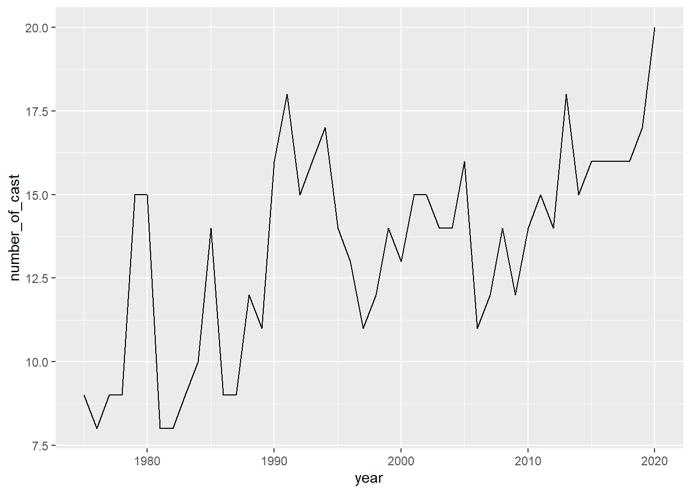
The graph shows that the number of casts appearing per season during SNL 46 seasons is gradually increasing.