Challenge 8

challenge_8
faostat
Joining Data
Author

Ananya Pujary

Published

August 25, 2022

library(tidyverse)
library(ggplot2)
library(summarytools)
library(dplyr)

knitr::opts_chunk$set(echo = TRUE, warning=FALSE, message=FALSE)

Read in data

Reading in the faostat datasets.

faostat_egg <- read_csv("_data/FAOSTAT_egg_chicken.csv")
faostat_livestock <- read_csv("_data/FAOSTAT_livestock.csv")
faostat_cattle <- read_csv("_data/FAOSTAT_cattle_dairy.csv")
faostat_country <- read_csv ("_data/FAOSTAT_country_groups.csv")

Briefly describe the data

print(summarytools::dfSummary(faostat_egg, varnumbers = FALSE, plain.ascii = FALSE, graph.magnif = 0.50, style = "grid", valid.col = FALSE), 
      method = 'render', table.classes = 'table-condensed')

Data Frame Summary

faostat_egg

Dimensions: 38170 x 14
Duplicates: 0
Variable Stats / Values Freqs (% of Valid) Graph Missing
Domain Code [character] 1. QL
38170(100.0%)
0 (0.0%)
Domain [character] 1. Livestock Primary
38170(100.0%)
0 (0.0%)
Area Code [numeric]
Mean (sd) : 771.1 (1709.6)
min ≤ med ≤ max:
1 ≤ 143 ≤ 5504
IQR (CV) : 145 (2.2)
245 distinct values 0 (0.0%)
Area [character]
1. Afghanistan
2. Africa
3. Albania
4. Algeria
5. American Samoa
6. Americas
7. Angola
8. Antigua and Barbuda
9. Argentina
10. Asia
[ 235 others ]
174(0.5%)
174(0.5%)
174(0.5%)
174(0.5%)
174(0.5%)
174(0.5%)
174(0.5%)
174(0.5%)
174(0.5%)
174(0.5%)
36430(95.4%)
0 (0.0%)
Element Code [numeric]
Mean (sd) : 5411.4 (80.5)
min ≤ med ≤ max:
5313 ≤ 5410 ≤ 5510
IQR (CV) : 197 (0)
5313:12679(33.2%)
5410:12651(33.1%)
5510:12840(33.6%)
0 (0.0%)
Element [character]
1. Laying
2. Production
3. Yield
12679(33.2%)
12840(33.6%)
12651(33.1%)
0 (0.0%)
Item Code [numeric] 1 distinct value
1062:38170(100.0%)
0 (0.0%)
Item [character] 1. Eggs, hen, in shell
38170(100.0%)
0 (0.0%)
Year Code [numeric]
Mean (sd) : 1990.5 (16.7)
min ≤ med ≤ max:
1961 ≤ 1991 ≤ 2018
IQR (CV) : 29 (0)
58 distinct values 0 (0.0%)
Year [numeric]
Mean (sd) : 1990.5 (16.7)
min ≤ med ≤ max:
1961 ≤ 1991 ≤ 2018
IQR (CV) : 29 (0)
58 distinct values 0 (0.0%)
Unit [character]
1. 1000 Head
2. 100mg/An
3. tonnes
12679(33.2%)
12651(33.1%)
12840(33.6%)
0 (0.0%)
Value [numeric]
Mean (sd) : 291341.2 (2232761)
min ≤ med ≤ max:
1 ≤ 31996 ≤ 76769955
IQR (CV) : 91235.8 (7.7)
21325 distinct values 40 (0.1%)
Flag [character]
1. *
2. A
3. F
4. Fc
5. Im
6. M
1435(4.7%)
3186(10.4%)
10538(34.4%)
13344(43.6%)
2079(6.8%)
40(0.1%)
7548 (19.8%)
Flag Description [character]
1. Aggregate, may include of
2. Calculated data
3. Data not available
4. FAO data based on imputat
5. FAO estimate
6. Official data
7. Unofficial figure
3186(8.3%)
13344(35.0%)
40(0.1%)
2079(5.4%)
10538(27.6%)
7548(19.8%)
1435(3.8%)
0 (0.0%)

Generated by summarytools 1.0.1 (R version 4.2.1)
2022-08-31

dim(faostat_egg)
[1] 38170    14

The faostat_egg dataset has 38170 rows and 13 columns. There are 40 missing values in the ‘Values’ column and 7548 missing values in ‘Flag’.

#| label: data description 2

print(summarytools::dfSummary(faostat_livestock, varnumbers = FALSE, plain.ascii = FALSE, graph.magnif = 0.50, style = "grid", valid.col = FALSE), 
      method = 'render', table.classes = 'table-condensed')

Data Frame Summary

faostat_livestock

Dimensions: 82116 x 14
Duplicates: 0
Variable Stats / Values Freqs (% of Valid) Graph Missing
Domain Code [character] 1. QA
82116(100.0%)
0 (0.0%)
Domain [character] 1. Live Animals
82116(100.0%)
0 (0.0%)
Area Code [numeric]
Mean (sd) : 912.7 (1855)
min ≤ med ≤ max:
1 ≤ 146 ≤ 5504
IQR (CV) : 148 (2)
253 distinct values 0 (0.0%)
Area [character]
1. Africa
2. Asia
3. China, mainland
4. Eastern Africa
5. Eastern Asia
6. Eastern Europe
7. Egypt
8. Europe
9. India
10. Northern Africa
[ 243 others ]
522(0.6%)
522(0.6%)
522(0.6%)
522(0.6%)
522(0.6%)
522(0.6%)
522(0.6%)
522(0.6%)
522(0.6%)
522(0.6%)
76896(93.6%)
0 (0.0%)
Element Code [numeric] 1 distinct value
5111:82116(100.0%)
0 (0.0%)
Element [character] 1. Stocks
82116(100.0%)
0 (0.0%)
Item Code [numeric]
Mean (sd) : 1017.7 (83.3)
min ≤ med ≤ max:
866 ≤ 1034 ≤ 1126
IQR (CV) : 120 (0.1)
866:13086(15.9%)
946:3505(4.3%)
976:11919(14.5%)
1016:12498(15.2%)
1034:12015(14.6%)
1096:11104(13.5%)
1107:8571(10.4%)
1110:6153(7.5%)
1126:3265(4.0%)
0 (0.0%)
Item [character]
1. Asses
2. Buffaloes
3. Camels
4. Cattle
5. Goats
6. Horses
7. Mules
8. Pigs
9. Sheep
8571(10.4%)
3505(4.3%)
3265(4.0%)
13086(15.9%)
12498(15.2%)
11104(13.5%)
6153(7.5%)
12015(14.6%)
11919(14.5%)
0 (0.0%)
Year Code [numeric]
Mean (sd) : 1990.4 (16.8)
min ≤ med ≤ max:
1961 ≤ 1991 ≤ 2018
IQR (CV) : 29 (0)
58 distinct values 0 (0.0%)
Year [numeric]
Mean (sd) : 1990.4 (16.8)
min ≤ med ≤ max:
1961 ≤ 1991 ≤ 2018
IQR (CV) : 29 (0)
58 distinct values 0 (0.0%)
Unit [character] 1. Head
82116(100.0%)
0 (0.0%)
Value [numeric]
Mean (sd) : 11625569 (64779790)
min ≤ med ≤ max:
0 ≤ 224667 ≤ 1489744504
IQR (CV) : 2364200 (5.6)
43667 distinct values 1301 (1.6%)
Flag [character]
1. *
2. A
3. F
4. Im
5. M
2667(6.1%)
12567(28.7%)
24550(56.0%)
2877(6.6%)
1185(2.7%)
38270 (46.6%)
Flag Description [character]
1. Aggregate, may include of
2. Data not available
3. FAO data based on imputat
4. FAO estimate
5. Official data
6. Unofficial figure
12567(15.3%)
1185(1.4%)
2877(3.5%)
24550(29.9%)
38270(46.6%)
2667(3.2%)
0 (0.0%)

Generated by summarytools 1.0.1 (R version 4.2.1)
2022-08-31

dim(faostat_livestock)
[1] 82116    14

There are 82116 rows and 13 columns in the faostat_livestock dataset. It has missing values too (1301 in ‘Value’ and 38270 in ‘Flag’).

#| label: data description 3

print(summarytools::dfSummary(faostat_country, varnumbers = FALSE, plain.ascii = FALSE, graph.magnif = 0.50, style = "grid", valid.col = FALSE), 
      method = 'render', table.classes = 'table-condensed')

Data Frame Summary

faostat_country

Dimensions: 1943 x 7
Duplicates: 0
Variable Stats / Values Freqs (% of Valid) Graph Missing
Country Group Code [numeric]
Mean (sd) : 5501.8 (1356.5)
min ≤ med ≤ max:
336 ≤ 5403 ≤ 9011
IQR (CV) : 648 (0.2)
58 distinct values 0 (0.0%)
Country Group [character]
1. World
2. Non-Annex I countries
3. Net Food Importing Develo
4. Annex I countries
5. High-income economies
6. Africa
7. Europe
8. Americas
9. Small Island Developing S
10. Upper-middle-income econo
[ 48 others ]
277(14.3%)
161(8.3%)
81(4.2%)
78(4.0%)
64(3.3%)
63(3.2%)
63(3.2%)
61(3.1%)
58(3.0%)
56(2.9%)
981(50.5%)
0 (0.0%)
Country Code [numeric]
Mean (sd) : 142.2 (96.4)
min ≤ med ≤ max:
1 ≤ 136 ≤ 622
IQR (CV) : 133 (0.7)
277 distinct values 0 (0.0%)
Country [character]
1. Afghanistan
2. Burkina Faso
3. Burundi
4. Central African Republic
5. Chad
6. Comoros
7. Ethiopia
8. Guinea-Bissau
9. Lesotho
10. Malawi
[ 267 others ]
11(0.6%)
11(0.6%)
11(0.6%)
11(0.6%)
11(0.6%)
11(0.6%)
11(0.6%)
11(0.6%)
11(0.6%)
11(0.6%)
1833(94.3%)
0 (0.0%)
M49 Code [character]
1. 004
2. 108
3. 140
4. 148
5. 174
6. 231
7. 426
8. 454
9. 466
10. 496
[ 267 others ]
11(0.6%)
11(0.6%)
11(0.6%)
11(0.6%)
11(0.6%)
11(0.6%)
11(0.6%)
11(0.6%)
11(0.6%)
11(0.6%)
1833(94.3%)
0 (0.0%)
ISO2 Code [character]
1. AF
2. BF
3. BI
4. CF
5. ET
6. GW
7. KM
8. LS
9. ML
10. MN
[ 266 others ]
11(0.6%)
11(0.6%)
11(0.6%)
11(0.6%)
11(0.6%)
11(0.6%)
11(0.6%)
11(0.6%)
11(0.6%)
11(0.6%)
1825(94.3%)
8 (0.4%)
ISO3 Code [character]
1. AFG
2. BDI
3. BFA
4. CAF
5. COM
6. ETH
7. GNB
8. LSO
9. MLI
10. MNG
[ 267 others ]
11(0.6%)
11(0.6%)
11(0.6%)
11(0.6%)
11(0.6%)
11(0.6%)
11(0.6%)
11(0.6%)
11(0.6%)
11(0.6%)
1833(94.3%)
0 (0.0%)

Generated by summarytools 1.0.1 (R version 4.2.1)
2022-08-31

dim(faostat_country)
[1] 1943    7

The faostat_country dataset has 1943 rows and 7 columns. It contains information on each country name and unique code, the country groups they belong to, as well as codes for ‘M49’, ‘ISO2’, and ‘ISO3’. Only the ‘ISO2’ column has 8 missing values.

Tidy Data

Tidying faostat_country

faostat_country seems tidy enough to work with.

Tidying faostat_egg

# turning 'Element' and 'Flag Description' into factor type

faostat_egg$Element <- as.factor(faostat_egg$Element)
faostat_egg$'Flag Description' <- as.factor(faostat_egg$'Flag Description')


# deleting 'Year Code'

faostat_egg <- faostat_egg %>%
  select(-'Year Code')

Tidying faostat_livestock

# turning 'Element' and 'Flag Description' into factor type
faostat_livestock$Element <- as.factor(faostat_livestock$Element)
faostat_livestock$'Flag Description' <- as.factor(faostat_livestock$'Flag Description')


# deleting 'Year Code'
faostat_livestock <- faostat_livestock %>%
  select(-'Year Code')

Tidying faostat_cattle

# turning 'Element' and 'Flag Description' into factor type

faostat_cattle$Element <- as.factor(faostat_cattle$Element)
faostat_cattle$'Flag Description' <- as.factor(faostat_cattle$'Flag Description')


# deleting 'Year Code'

faostat_cattle <- faostat_cattle %>%
  select(-'Year Code')

Join Data

Be sure to include a sanity check, and double-check that case count is correct!

Joining faostat_egg and faostat_livestock by rowbinding:

egg_livestock <- bind_rows(faostat_egg,faostat_livestock)

dim(egg_livestock)
[1] 120286     13

Both datasets had 13 columns and the combined number of rows in the new dataset is \[38170 + 82116 = 120286\].

Joining faostat_cattle and faostat_livestockby rowbinding:

cattle_livestock <- bind_rows(faostat_cattle,faostat_livestock)

dim(cattle_livestock)
[1] 118565     13

Both datasets had 13 columns and the combined number of rows in the new dataset is \[36449 + 82116 = 118565\].

#figuring out the primary key for 'faostat_country'
faostat_country %>% 
  count('Country Code') %>% 
  filter(n > 1)
# A tibble: 1 × 2
  `"Country Code"`     n
  <chr>            <int>
1 Country Code      1943
faostat_country
# A tibble: 1,943 × 7
   `Country Group Code` `Country Group` Countr…¹ Country M49 C…² ISO2 …³ ISO3 …⁴
                  <dbl> <chr>              <dbl> <chr>   <chr>   <chr>   <chr>  
 1                 5100 Africa                 4 Algeria 012     DZ      DZA    
 2                 5100 Africa                 7 Angola  024     AO      AGO    
 3                 5100 Africa                53 Benin   204     BJ      BEN    
 4                 5100 Africa                20 Botswa… 072     BW      BWA    
 5                 5100 Africa               233 Burkin… 854     BF      BFA    
 6                 5100 Africa                29 Burundi 108     BI      BDI    
 7                 5100 Africa                35 Cabo V… 132     CV      CPV    
 8                 5100 Africa                32 Camero… 120     CM      CMR    
 9                 5100 Africa                37 Centra… 140     CF      CAF    
10                 5100 Africa                39 Chad    148     TD      TCD    
# … with 1,933 more rows, and abbreviated variable names ¹​`Country Code`,
#   ²​`M49 Code`, ³​`ISO2 Code`, ⁴​`ISO3 Code`
# ℹ Use `print(n = ...)` to see more rows
egg_livestock %>% 
  count('Area Code') %>% 
  filter(n > 1)
# A tibble: 1 × 2
  `"Area Code"`      n
  <chr>          <int>
1 Area Code     120286
unique(faostat_country$`Country Code`)
  [1]   4   7  53  20 233  29  35  32  37  39  24  45  46 107 250  72  59  61
 [19] 178 209 238  62  71  74  75  81  90 175 114 122 123 124 129 130 133 136
 [37] 137 270 143 144 147 158 159 182 184 187 193 195 196 197 201 202 277 276
 [55] 206 217 222 226 215 616 205 251 181 258   8   9  22  12  14  23  17  19
 [73] 278  31  21 239  33 609  36  40  44  48  49 279  55  56  58  60  65  69
 [91]  85  86  87  89  91  93  95 109 135 138 142 151 157 622 166 169 170 177
[109] 282 188 189 190 191 281 280 614 271 207 220 224 231 240 234 236   5  10
[127]  11  57 255  15  27 259  98  50 167  51  54  63  64  67  68  70  79  82
[145]  84  88  97  99 104 264 106 110 119 125 126 256 134 140 150 153 156 161
[163] 163 162 172 173 174 183 185 199 198 203 260 210 211 218 223 230 229 228
[181] 243  30   2   1  52  13  16  18  26 115 351  96 128  41 214 116  73 100
[199] 101 102 103 105 112 108 118 113 120 121 131 132 141  28 149 221 165 299
[217] 171 179 117 194 200  38 212 208 216 176 213 225 235 237 249 246 247  42
[235]  43  92 146 284   3   6  80  78  77 274  94 283 275 273 154 619 192 272
[253] 186 620 621 248 180  83  25 227 155 145 168  66 127 617 148 164 232  47
[271] 160 244 219 111 139 618 242
unique(egg_livestock$`Area Code`)
  [1]    2    3    4    5    7    8    9    1   10   11   52   12   13   16   14
 [16]   57  255   15   23   53   17   18   19   80   20   21   26   27  233   29
 [31]   35  115   32   33   36   37   39   40   96  128   41  214   44   45   46
 [46]   47   48  107   98   49   50  167   51  116  250   54   55   56   58   59
 [61]   60   61  178   63  209  238   62   66   67   68   69   70   74   75   73
 [76]   79   81   84   86   87   88   89   90  175   91   93   95   97   99  100
 [91]  101  102  103  104  105  106  109  110  112  108  114   83  118  113  120
[106]  119  121  122  123  124  125  126  256  129  130  131  133  134  135  136
[121]  137  138  145  141  273  142  143  144   28  147  148  149  150  151  153
[136]  156  157  158  159  160  154  162  221  164  165  299  166  168  169  170
[151]  171  173  174  177  179  117  146  182  183  185  184  188  189  190  191
[166]  244  193  194  195  272  186  196  197  200  199  198   25  201  202  277
[181]  203   38  276  206  207  210  211  212  208  216  176  217  218  219  220
[196]  222  223  213  227  226  230  225  229  215  231  240  234  228  235  155
[211]  236  237  243  249  248  251  181 5000 5100 5101 5102 5103 5104 5105 5200
[226] 5203 5204 5206 5207 5300 5301 5302 5303 5304 5305 5400 5401 5402 5403 5404
[241] 5500 5501 5502 5503 5504   22  239   72   65   64   85  161  187  205

So ‘Country Code’ can be used as the primary key for the faostat_country dataset to connect to the egg_livestock dataset.

join_anti <- egg_livestock %>%
  anti_join(faostat_country, by = c("Area Code"="Country Code")) 

dim(join_anti)
[1] 17346    13
unique(join_anti$`Area Code`)
 [1] 5000 5100 5101 5102 5103 5104 5105 5200 5203 5204 5206 5207 5300 5301 5302
[16] 5303 5304 5305 5400 5401 5402 5403 5404 5500 5501 5502 5503 5504
unique(egg_livestock$`Area Code`)
  [1]    2    3    4    5    7    8    9    1   10   11   52   12   13   16   14
 [16]   57  255   15   23   53   17   18   19   80   20   21   26   27  233   29
 [31]   35  115   32   33   36   37   39   40   96  128   41  214   44   45   46
 [46]   47   48  107   98   49   50  167   51  116  250   54   55   56   58   59
 [61]   60   61  178   63  209  238   62   66   67   68   69   70   74   75   73
 [76]   79   81   84   86   87   88   89   90  175   91   93   95   97   99  100
 [91]  101  102  103  104  105  106  109  110  112  108  114   83  118  113  120
[106]  119  121  122  123  124  125  126  256  129  130  131  133  134  135  136
[121]  137  138  145  141  273  142  143  144   28  147  148  149  150  151  153
[136]  156  157  158  159  160  154  162  221  164  165  299  166  168  169  170
[151]  171  173  174  177  179  117  146  182  183  185  184  188  189  190  191
[166]  244  193  194  195  272  186  196  197  200  199  198   25  201  202  277
[181]  203   38  276  206  207  210  211  212  208  216  176  217  218  219  220
[196]  222  223  213  227  226  230  225  229  215  231  240  234  228  235  155
[211]  236  237  243  249  248  251  181 5000 5100 5101 5102 5103 5104 5105 5200
[226] 5203 5204 5206 5207 5300 5301 5302 5303 5304 5305 5400 5401 5402 5403 5404
[241] 5500 5501 5502 5503 5504   22  239   72   65   64   85  161  187  205
check1 <- join_anti %>% 
  select(`Area Code`,`Area`) %>% 
  group_by(`Area Code`,`Area`) %>% 
  tally()
check1
# A tibble: 28 × 3
# Groups:   Area Code [28]
   `Area Code` Area                 n
         <dbl> <chr>            <int>
 1        5000 World              696
 2        5100 Africa             696
 3        5101 Eastern Africa     696
 4        5102 Middle Africa      638
 5        5103 Northern Africa    696
 6        5104 Southern Africa    638
 7        5105 Western Africa     638
 8        5200 Americas           638
 9        5203 Northern America   580
10        5204 Central America    580
# … with 18 more rows
# ℹ Use `print(n = ...)` to see more rows

The anti_join() on egg_livestock and faostat_country reveals that there are 17346 observations in egg_livestock that did not find a match in faostat_country. join_anti has 13 columns, the same as the egg_livestock dataset.

Analyze Data

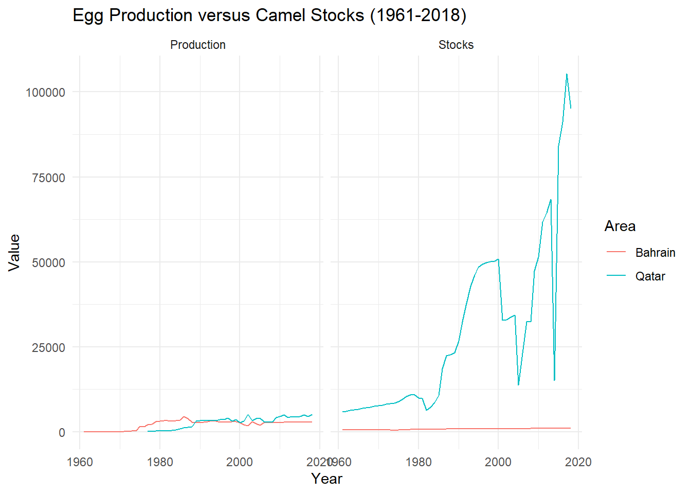
I’m looking to compare egg production to camel livestock production in Bahrain and Qatar using a line graph with facet wrap.

egg_livestock_filt <- egg_livestock %>%
  select(Year,Area,Item,Element,Value) %>%
  filter(Area=="Bahrain"|Area=="Qatar") %>%
  filter(Element=="Production"| Item=="Camels")
egg_livestock_filt
# A tibble: 216 × 5
    Year Area    Item                Element    Value
   <dbl> <chr>   <chr>               <fct>      <dbl>
 1  1961 Bahrain Eggs, hen, in shell Production    60
 2  1962 Bahrain Eggs, hen, in shell Production    60
 3  1963 Bahrain Eggs, hen, in shell Production    60
 4  1964 Bahrain Eggs, hen, in shell Production    60
 5  1965 Bahrain Eggs, hen, in shell Production    70
 6  1966 Bahrain Eggs, hen, in shell Production    70
 7  1967 Bahrain Eggs, hen, in shell Production    80
 8  1968 Bahrain Eggs, hen, in shell Production    80
 9  1969 Bahrain Eggs, hen, in shell Production    80
10  1970 Bahrain Eggs, hen, in shell Production    80
# … with 206 more rows
# ℹ Use `print(n = ...)` to see more rows
egg_livestock_filt %>%
  ggplot(aes(x=Year, y=Value, color=Area)) +
    geom_line() + labs(title = "Egg Production versus Camel Stocks (1961-2018)", x = "Year", y = "Value") + facet_wrap(~ Element) + theme_minimal()

Over time, egg production in Qatar exceeded that in Bahrain. Camel livestock production in Qatar evidently far-exceeds stocks in Bahrain too.