library(tidyverse)
library(ggplot2)
library(lubridate)

knitr::opts_chunk$set(echo = TRUE, warning=FALSE, message=FALSE)Challenge 8
challenge_8
snl
Joining Data
Introduction
This is a fun one! Today I am going to be joining, mutating, and analyzing data of SNL cast members and seasons.
Read in data
The data for this challenge are contained within three related .csv files.
snl_actors_orig<-read_csv("_data/snl_actors.csv")
snl_casts_orig<-read_csv("_data/snl_casts.csv")
snl_seasons_orig<-read_csv("_data/snl_seasons.csv")
Briefly describe the data
snl_actors_orig# A tibble: 2,306 × 4
aid url type gender
<chr> <chr> <chr> <chr>
1 Kate McKinnon /Cast/?KaMc cast female
2 Alex Moffat /Cast/?AlMo cast male
3 Ego Nwodim /Cast/?EgNw cast unknown
4 Chris Redd /Cast/?ChRe cast male
5 Kenan Thompson /Cast/?KeTh cast male
6 Carey Mulligan /Guests/?3677 guest andy
7 Marcus Mumford /Guests/?3679 guest male
8 Aidy Bryant /Cast/?AiBr cast female
9 Steve Higgins /Crew/?StHi crew male
10 Mikey Day /Cast/?MiDa cast male
# … with 2,296 more rows
# ℹ Use `print(n = ...)` to see more rowssnl_casts_orig# A tibble: 614 × 8
aid sid featured first_epid last_epid update…¹ n_epi…² seaso…³
<chr> <dbl> <lgl> <dbl> <dbl> <lgl> <dbl> <dbl>
1 A. Whitney Brown 11 TRUE 19860222 NA FALSE 8 0.444
2 A. Whitney Brown 12 TRUE NA NA FALSE 20 1
3 A. Whitney Brown 13 TRUE NA NA FALSE 13 1
4 A. Whitney Brown 14 TRUE NA NA FALSE 20 1
5 A. Whitney Brown 15 TRUE NA NA FALSE 20 1
6 A. Whitney Brown 16 TRUE NA NA FALSE 20 1
7 Alan Zweibel 5 TRUE 19800409 NA FALSE 5 0.25
8 Sasheer Zamata 39 TRUE 20140118 NA FALSE 11 0.524
9 Sasheer Zamata 40 TRUE NA NA FALSE 21 1
10 Sasheer Zamata 41 FALSE NA NA FALSE 21 1
# … with 604 more rows, and abbreviated variable names ¹update_anchor,
# ²n_episodes, ³season_fraction
# ℹ Use `print(n = ...)` to see more rowssnl_seasons_orig# A tibble: 46 × 5
sid year first_epid last_epid n_episodes
<dbl> <dbl> <dbl> <dbl> <dbl>
1 1 1975 19751011 19760731 24
2 2 1976 19760918 19770521 22
3 3 1977 19770924 19780520 20
4 4 1978 19781007 19790526 20
5 5 1979 19791013 19800524 20
6 6 1980 19801115 19810411 13
7 7 1981 19811003 19820522 20
8 8 1982 19820925 19830514 20
9 9 1983 19831008 19840512 19
10 10 1984 19841006 19850413 17
# … with 36 more rows
# ℹ Use `print(n = ...)` to see more rowsThe “actors” dataframe appears to record every individual who has made an appearance on Saturday Night Live, whether that was as a cast member, a guest (including musical guests), or someone with a “crew” designation (the meaning of which is not entirely clear). The urls aren’t very pretty, so I will remove them from the dataframe at the tidying stage.
The “casts” dataframe focusses on individuals who have appeared as cast members on the show, excluding guests from the list. Specification is made for whether or not a cast member was a featured player (a designation below a full repertory cast member) for a given season, as well as whether or not they served as a “Weekend Update” anchor. In certain cases, this dataframe will also give the date of the first and/or last episode on which a given cast member appeared; however, these cases are inconsistent at best. With this being the case, and given the analysis I intend to do, I will be removing these first and last episode columns when I tidy the data. I will also delete and recreate the season_fraction column, just to make sure all values are correct with no mistakes.
Lastly, the “seasons” dataframe is a simple table of basic data for every season of SNL. This table has its own first and last episode dates, for the start and end of each season; these columns are consistent throughout, and I will keep them in the dataframe.
Tidying Data
In my own exploratory analysis, I had done most of my tidying and joining together, but both for the sake of clarity and of being careful I will split up those steps here.
The only real tidying that needs to be done on these dataframes is the removal or cleanup of pesky columns; the data themselves are all tidy. (Recreating the sesason_fraction variable will actually not come until the data are joined.) Additionally, two of the dataframes have columns named “n_episodes” which track different variables, so I will rename these to prepare for clean joining.
snl_actors<-snl_actors_orig %>%
  select(-url)

snl_casts<-snl_casts_orig %>%
  select(-c(contains("epid"),season_fraction)) %>%
  rename("n_episodes_player"="n_episodes")

snl_seasons<-snl_seasons_orig %>%
  mutate(first_epid=ymd(first_epid)) %>%
  mutate(last_epid=ymd(last_epid)) %>%
  rename("n_episodes_season"="n_episodes")

head(snl_actors)
# A tibble: 6 × 3
aid type gender
<chr> <chr> <chr>
1 Kate McKinnon cast female
2 Alex Moffat cast male
3 Ego Nwodim cast unknown
4 Chris Redd cast male
5 Kenan Thompson cast male
6 Carey Mulligan guest andy head(snl_casts)# A tibble: 6 × 5
aid sid featured update_anchor n_episodes_player
<chr> <dbl> <lgl> <lgl> <dbl>
1 A. Whitney Brown 11 TRUE FALSE 8
2 A. Whitney Brown 12 TRUE FALSE 20
3 A. Whitney Brown 13 TRUE FALSE 13
4 A. Whitney Brown 14 TRUE FALSE 20
5 A. Whitney Brown 15 TRUE FALSE 20
6 A. Whitney Brown 16 TRUE FALSE 20head(snl_seasons)# A tibble: 6 × 5
sid year first_epid last_epid n_episodes_season
<dbl> <dbl> <date> <date> <dbl>
1 1 1975 1975-10-11 1976-07-31 24
2 2 1976 1976-09-18 1977-05-21 22
3 3 1977 1977-09-24 1978-05-20 20
4 4 1978 1978-10-07 1979-05-26 20
5 5 1979 1979-10-13 1980-05-24 20
6 6 1980 1980-11-15 1981-04-11 13Join Data
Keys and Case Counts
Before we start joining data, we want to make sure we know what the case counts are for each dataframe, and also make sure that we know which variables or combinations of variables serve as the unique keys for each dataframe.
“snl_actors” has 2306 rows and 3 columns. “snl_casts” has 614 rows and 5 columns. “snl_seasons” has 46 rows and 5 columns.
snl_actors %>%
  count(aid) %>%
  filter(n>1)
# A tibble: 0 × 2
# … with 2 variables: aid <chr>, n <int>
# ℹ Use `colnames()` to see all variable namessnl_casts %>%
count(aid,sid) %>%
filter(n>1)# A tibble: 0 × 3
# … with 3 variables: aid <chr>, sid <dbl>, n <int>
# ℹ Use `colnames()` to see all variable namessnl_seasons %>%
count(sid) %>%
filter(n>1)# A tibble: 0 × 2
# … with 2 variables: sid <dbl>, n <int>
# ℹ Use `colnames()` to see all variable namesThe unique keys are the variables “aid” (actor ID) for snl_actors and “sid” (season ID) for snl_seasons, with the snl_casts dataframe taking each joint aid-sid case as its unique key.
Joins
snl_casts and snl_seasons
It would be interesting to see the information from the snl_seasons dataframe listed on the snl_casts dataframe. This can be accomplished with a simple join.
Before we perform this join, we can preemptively do a simple sanity check. These dataframes only share one key – the “sid” variable – so the final joined dataframe will have as many columns as snl_casts and snl_seasons combined, less one – without adding any rows. In other words, this means that we should end up with 614 rows and 9 columns.
nrow(snl_casts)[1] 614ncol(snl_casts) + ncol(snl_seasons) - 1[1] 9snl_casts_seas <- snl_casts %>%
left_join(snl_seasons,by="sid")
snl_casts_seas# A tibble: 614 × 9
aid sid featu…¹ updat…² n_epi…³ year first_epid last_epid n_epi…⁴
<chr> <dbl> <lgl> <lgl> <dbl> <dbl> <date> <date> <dbl>
1 A. Whitney… 11 TRUE FALSE 8 1985 1985-11-09 1986-05-24 18
2 A. Whitney… 12 TRUE FALSE 20 1986 1986-10-11 1987-05-23 20
3 A. Whitney… 13 TRUE FALSE 13 1987 1987-10-17 1988-02-27 13
4 A. Whitney… 14 TRUE FALSE 20 1988 1988-10-08 1989-05-20 20
5 A. Whitney… 15 TRUE FALSE 20 1989 1989-09-30 1990-05-19 20
6 A. Whitney… 16 TRUE FALSE 20 1990 1990-09-29 1991-05-18 20
7 Alan Zweib… 5 TRUE FALSE 5 1979 1979-10-13 1980-05-24 20
8 Sasheer Za… 39 TRUE FALSE 11 2013 2013-09-28 2014-05-17 21
9 Sasheer Za… 40 TRUE FALSE 21 2014 2014-09-27 2015-05-16 21
10 Sasheer Za… 41 FALSE FALSE 21 2015 2015-10-03 2016-05-21 21
# … with 604 more rows, and abbreviated variable names ¹featured,
# ²update_anchor, ³n_episodes_player, ⁴n_episodes_season
# ℹ Use `print(n = ...)` to see more rowsdim(snl_casts_seas)[1] 614 9Perfect!
Now that we’ve completed this join, we can recreate what had been called the “season_fraction” variable in the snl_casts_orig dataframe. This variable recorded the percentage of a given season’s episodes in which a given player appeared. For clarity, I am going to call this variable the “player_appearance_rate” in this dataframe.
snl_casts_seas<-snl_casts_seas %>%
  mutate(player_appearance_rate=(n_episodes_player/n_episodes_season))

snl_casts_seas
# A tibble: 614 × 10
aid sid featu…¹ updat…² n_epi…³ year first_epid last_epid n_epi…⁴
<chr> <dbl> <lgl> <lgl> <dbl> <dbl> <date> <date> <dbl>
1 A. Whitney… 11 TRUE FALSE 8 1985 1985-11-09 1986-05-24 18
2 A. Whitney… 12 TRUE FALSE 20 1986 1986-10-11 1987-05-23 20
3 A. Whitney… 13 TRUE FALSE 13 1987 1987-10-17 1988-02-27 13
4 A. Whitney… 14 TRUE FALSE 20 1988 1988-10-08 1989-05-20 20
5 A. Whitney… 15 TRUE FALSE 20 1989 1989-09-30 1990-05-19 20
6 A. Whitney… 16 TRUE FALSE 20 1990 1990-09-29 1991-05-18 20
7 Alan Zweib… 5 TRUE FALSE 5 1979 1979-10-13 1980-05-24 20
8 Sasheer Za… 39 TRUE FALSE 11 2013 2013-09-28 2014-05-17 21
9 Sasheer Za… 40 TRUE FALSE 21 2014 2014-09-27 2015-05-16 21
10 Sasheer Za… 41 FALSE FALSE 21 2015 2015-10-03 2016-05-21 21
# … with 604 more rows, 1 more variable: player_appearance_rate <dbl>, and
# abbreviated variable names ¹featured, ²update_anchor, ³n_episodes_player,
# ⁴n_episodes_season
# ℹ Use `print(n = ...)` to see more rows, and `colnames()` to see all variable namesObservations
Having performed these joins and mutations, we can find some interesting information. For example, which cast member had the lowest average appearance rate over the course of their career?
snl_casts_seas %>%
  group_by(aid) %>%
  summarise(mean_app_rate=mean(player_appearance_rate)) %>%
  arrange(mean_app_rate) %>%
  slice(1:10)
# A tibble: 10 × 2
aid mean_app_rate
<chr> <dbl>
1 George Coe 0.0417
2 Emily Prager 0.0769
3 Laurie Metcalf 0.0769
4 Michael O'Donoghue 0.167
5 Morwenna Banks 0.2
6 Alan Zweibel 0.25
7 Tom Schiller 0.25
8 Ben Stiller 0.3
9 Tony Rosato 0.538
10 Fred Wolf 0.575 The answer is George Coe, who is an interesting case of having only been credited for his appearance in the very first episode of SNL, despite featuring in various subsequent episodes as well.
We can also visualize how the average appearance rate changed from season to season.
snl_casts_seas %>%
  group_by(year) %>%
  summarize(mean_seas_app_rate=mean(player_appearance_rate)) %>%
  ggplot(aes(year,mean_seas_app_rate)) +
  geom_point() +
  geom_line() +
  theme_bw() +
  scale_y_continuous(labels = scales::percent) +
  labs(title="Average Player Apperance Rate by Year",
       x="Year",
       y="Average Player Appearance Rate")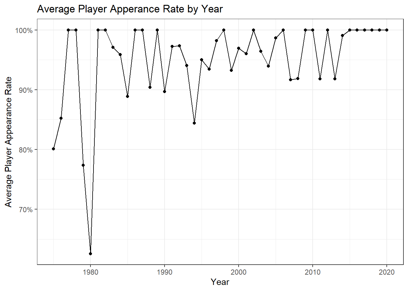
It is very interesting to observe that the last six seasons have all had every player feature in every episode! It is also interesting to observe the distinct drop in 1979 and 1980, and I wonder at the reasons behind this drop.