library(tidyverse)
library(ggplot2)
library(lubridate)
library(ggridges)

knitr::opts_chunk$set(echo = TRUE, warning=FALSE, message=FALSE)Did Racing Improve During Formula 1’s Hybrid Era?
final
Comparing the 2014-2021 Formula 1 World Championships to Previous Seasons Using the R Statistical Package
Introduction
The Formula 1 World Championship is the world’s premier motorsports competition. F1 Grands Prix are held in a number of countries every year, and millions of fans are attracted from even farther afield. As if racing at 200 mph wasn’t enough, competition is just about as competitive off the track as it is on it, with each of the Championship’s ten constructors constantly innovating and engineering along the cutting edge of what is possible – and what is allowed – in their pursuit of racing perfection.
One of the most groundbreaking innovations in recent F1 history was the start of what has come to be known as the Hybrid Era, in 2014. The Hybrid Era, which lasted until the end of the 2021 season, saw a sweeping series of rule changes that forced constructors to transition from cars powered solely by internal combustion to ones with hybrid “power units,” combining turbo-charged engines with battery power as well as “energy recovery systems” that regenerate power from the energy lost in braking and other functions.
Research Question
The intent of this analysis is to examine at a preliminary level whether or not lap time data from before and during F1’s Hybrid Era suggest that racing improved over the course of the Hybrid Era, with shorter lap times indicating improvement. It is important to note that faster lap times are an imperfect gauge for improvement in racing overall. Of course, a general trend toward shorter lap times would suggest higher (average) speeds and overall faster racing, as well as technological advancement when observed across the 20-car grid. However, such faster times could also be a symptom of racing with fewer overtakes, which is generally considered uninteresting and is a problem that Formula 1 has needed to address throughout the Hybrid Era. However, for the sake of simplicity, this analysis will focus on lap times. A more complete analysis would factor in overtaking data from before and during the Hybrid Era to gain a more complete understanding of the state of racing in F1.
Data
The data I’m using is the “Formula 1 World Championship (1950-2022)” dataset available on Kaggle from Rohan Rao, under the username Vopani, who in turn collected the data from an online API known by the name of “Ergast”. This dataset is a collection of .csv files, each detailing a certain aspect of race data, which can be joined easily for more in-depth analysis.
For my analysis, I will only be using four of these .csv files:
races.csv, which holds identifying data about races referenced across the entire dataset;circuits.csv, which similarly holds identifying data about every circuit;qualifying.csv, which holds lap time data for racers’ best laps across all three qualifying rounds for every Grand Prix in the data set; and,lap_times.csv, which holds lap time data for every racer’s every lap across all Grands Prix included.
# races.csv

master_races<-read_csv(
  file="_data/f1archive/races.csv",
  skip=1,
  col_select=1:6,
  col_names=c("race_id","seas_year","seas_round","circ_id","name_race","date_race")
)

master_races
# A tibble: 1,079 × 6
race_id seas_year seas_round circ_id name_race date_race
<dbl> <dbl> <dbl> <dbl> <chr> <date>
1 1 2009 1 1 Australian Grand Prix 2009-03-29
2 2 2009 2 2 Malaysian Grand Prix 2009-04-05
3 3 2009 3 17 Chinese Grand Prix 2009-04-19
4 4 2009 4 3 Bahrain Grand Prix 2009-04-26
5 5 2009 5 4 Spanish Grand Prix 2009-05-10
6 6 2009 6 6 Monaco Grand Prix 2009-05-24
7 7 2009 7 5 Turkish Grand Prix 2009-06-07
8 8 2009 8 9 British Grand Prix 2009-06-21
9 9 2009 9 20 German Grand Prix 2009-07-12
10 10 2009 10 11 Hungarian Grand Prix 2009-07-26
# … with 1,069 more rows
# ℹ Use `print(n = ...)` to see more rows# circuits.csv
master_circ<-read_csv(
file="_data/f1archive/circuits.csv",
col_select=1:8,
skip=1,
col_types="nccccnnn",
col_names=c("circ_id","circ_ref","circ_name","circ_loc","circ_nat",
"circ_lat","circ_lng","circ_alt")
)
master_circ# A tibble: 76 × 8
circ_id circ_ref circ_name circ_…¹ circ_…² circ_…³ circ_…⁴ circ_…⁵
<dbl> <chr> <chr> <chr> <chr> <dbl> <dbl> <dbl>
1 1 albert_park Albert Park G… Melbou… Austra… -37.8 145. 10
2 2 sepang Sepang Intern… Kuala … Malays… 2.76 102. 18
3 3 bahrain Bahrain Inter… Sakhir Bahrain 26.0 50.5 7
4 4 catalunya Circuit de Ba… Montme… Spain 41.6 2.26 109
5 5 istanbul Istanbul Park Istanb… Turkey 41.0 29.4 130
6 6 monaco Circuit de Mo… Monte-… Monaco 43.7 7.42 7
7 7 villeneuve Circuit Gille… Montre… Canada 45.5 -73.5 13
8 8 magny_cours Circuit de Ne… Magny … France 46.9 3.16 228
9 9 silverstone Silverstone C… Silver… UK 52.1 -1.02 153
10 10 hockenheimring Hockenheimring Hocken… Germany 49.3 8.57 103
# … with 66 more rows, and abbreviated variable names ¹circ_loc, ²circ_nat,
# ³circ_lat, ⁴circ_lng, ⁵circ_alt
# ℹ Use `print(n = ...)` to see more rows# qualifying.csv
qual<-read_csv(
file="_data/f1archive/qualifying.csv",
skip=1,
col_names=c("qual_id","race_id","driv_id","con_id","driv_num","qual_pos","q1","q2","q3")
)
qual_race<-qual %>%
mutate(q1=ms(q1)) %>%
mutate(q2=ms(q2)) %>%
mutate(q3=ms(q3)) %>%
pivot_longer(
cols = q1:q3,
names_to = "qual_round",
values_to = "qual_time"
) %>%
mutate(qual_round=str_remove_all(qual_round,"[q]")) %>%
mutate(qual_round=as.numeric(qual_round)) %>%
left_join(master_races) %>%
left_join(master_circ)
qual_race# A tibble: 28,185 × 20
qual_id race_id driv_id con_id driv_num qual_pos qual_ro…¹ qual_time seas_…²
<dbl> <dbl> <dbl> <dbl> <dbl> <dbl> <dbl> <Period> <dbl>
1 1 18 1 1 22 1 1 1M 26.572S 2008
2 1 18 1 1 22 1 2 1M 25.187S 2008
3 1 18 1 1 22 1 3 1M 26.714S 2008
4 2 18 9 2 4 2 1 1M 26.103S 2008
5 2 18 9 2 4 2 2 1M 25.315S 2008
6 2 18 9 2 4 2 3 1M 26.869S 2008
7 3 18 5 1 23 3 1 1M 25.664S 2008
8 3 18 5 1 23 3 2 1M 25.452S 2008
9 3 18 5 1 23 3 3 1M 27.079S 2008
10 4 18 13 6 2 4 1 1M 25.994S 2008
# … with 28,175 more rows, 11 more variables: seas_round <dbl>, circ_id <dbl>,
# name_race <chr>, date_race <date>, circ_ref <chr>, circ_name <chr>,
# circ_loc <chr>, circ_nat <chr>, circ_lat <dbl>, circ_lng <dbl>,
# circ_alt <dbl>, and abbreviated variable names ¹qual_round, ²seas_year
# ℹ Use `print(n = ...)` to see more rows, and `colnames()` to see all variable names# lap_times.csv
lap_times<-read_csv(
file="_data/f1archive/lap_times.csv",
skip=1,
col_names=c("race_id","driv_id","lap","pos_race","time_lap_char","time_lap_ms"),
col_types="nnnncn"
)
lap_times<-lap_times %>%
mutate(time_lap=ms(time_lap_char)) %>%
select(-"time_lap_char") %>%
left_join(master_races) %>%
left_join(master_circ)
lap_times# A tibble: 528,785 × 18
race_id driv_id lap pos_race time_lap_ms time_lap seas_…¹ seas_…² circ_id
<dbl> <dbl> <dbl> <dbl> <dbl> <Period> <dbl> <dbl> <dbl>
1 841 20 1 1 98109 1M 38.109S 2011 1 1
2 841 20 2 1 93006 1M 33.006S 2011 1 1
3 841 20 3 1 92713 1M 32.713S 2011 1 1
4 841 20 4 1 92803 1M 32.803S 2011 1 1
5 841 20 5 1 92342 1M 32.342S 2011 1 1
6 841 20 6 1 92605 1M 32.605S 2011 1 1
7 841 20 7 1 92502 1M 32.502S 2011 1 1
8 841 20 8 1 92537 1M 32.537S 2011 1 1
9 841 20 9 1 93240 1M 33.24S 2011 1 1
10 841 20 10 1 92572 1M 32.572S 2011 1 1
# … with 528,775 more rows, 9 more variables: name_race <chr>,
# date_race <date>, circ_ref <chr>, circ_name <chr>, circ_loc <chr>,
# circ_nat <chr>, circ_lat <dbl>, circ_lng <dbl>, circ_alt <dbl>, and
# abbreviated variable names ¹seas_year, ²seas_round
# ℹ Use `print(n = ...)` to see more rows, and `colnames()` to see all variable namesfastest_laps<-lap_times %>%
group_by(race_id) %>%
summarise(time_lap_ms=min(time_lap_ms)) %>%
left_join(lap_times) %>%
left_join(master_races)
fastest_laps<-fastest_laps %>%
filter(seas_year>=2002) %>%
count(circ_id,name_race) %>%
filter(n>=10) %>%
left_join(fastest_laps) %>%
select(!n) %>%
filter(race_id!=1063) %>% # One-off race at modified Bahrain circuit
left_join(master_circ)
fastest_laps# A tibble: 363 × 18
circ_id name_race race_id time_…¹ driv_id lap pos_r…² time_lap seas_…³
<dbl> <chr> <dbl> <dbl> <dbl> <dbl> <dbl> <Period> <dbl>
1 1 Australian … 1 87706 3 48 7 1M 27.706S 2009
2 1 Australian … 18 87418 5 43 1 1M 27.418S 2008
3 1 Australian … 36 85235 8 41 1 1M 25.235S 2007
4 1 Australian … 55 86045 8 57 2 1M 26.045S 2006
5 1 Australian … 71 85683 4 24 3 1M 25.683S 2005
6 1 Australian … 90 84125 30 29 1 1M 24.125S 2004
7 1 Australian … 108 87724 8 32 1 1M 27.724S 2003
8 1 Australian … 124 88541 8 37 2 1M 28.541S 2002
9 1 Australian … 141 88214 30 34 1 1M 28.214S 2001
10 1 Australian … 158 91481 22 41 2 1M 31.481S 2000
# … with 353 more rows, 9 more variables: seas_round <dbl>, date_race <date>,
# circ_ref <chr>, circ_name <chr>, circ_loc <chr>, circ_nat <chr>,
# circ_lat <dbl>, circ_lng <dbl>, circ_alt <dbl>, and abbreviated variable
# names ¹time_lap_ms, ²pos_race, ³seas_year
# ℹ Use `print(n = ...)` to see more rows, and `colnames()` to see all variable namesThese .csv files are for the most part already “Tidy” according to the Tidyverse understanding of data wrangling and analysis. Beyond superficial column-name changes, the most significant data cleanup act took place on the qualifying data, where I pivoted the rounds 1-3 columns longer into a “round” and a “lap time” column. Additionally, I joined both the qualifying and the lap times dataframes with the races and circuits master dataframes, for more complete identification.
I ended up taking two dataframes out of the lap_times.csv data set. The first, lap_times, retains the data in its original form, joins notwithstanding. The second, fastest_laps, uses a group_by()/summarise() combo to isolate the fastest laps (minimum lap time) for each Grand Prix. This isolated fastest lap data plays a crucial role on its own in the analysis to follow.
Visualizations
The analysis of these Formula 1 data were performed using the ggplot2 package from the Tidyverse collection of R-language packages. Again, these analyses are largely preliminary and exploratory, and were not verified with statistically rigorous hypotheses tests. They do, however, lay a solid foundation for such research to be performed in the future.
What follows are three ggplot visualizations of qualifying and race lap time data drawn from Grands Prix held at nine different circuits between 1996 and 2021. The nine circuits chosen were selected based on the frequency of their use in an unchanging configuration; certain Formula 1-eligible circuits are not used regularly or even very often at all, while others have undergone significant alterations in their configuration, making lap time comparisons meaningless. The wide date range gives enough lead time to establish a visual baseline with which to compare the Hybrid Era seasons of 2014 to 2021.
The selected nine circuits (along with their country and/or more familiar name) are:
- Albert Park (Australia)
- Autodromo Jose Carlos Pace (Interlagos/Sao Paolo, Brazil)
- Monza (Italy)
- Barcelona (Spain)
- Monaco
- Gilles Villneuve (Canada)
- Hungaroring (Hungary)
- Sepang (Malaysia)
- Suzuka (Japan)
Fastest Laps
The first of these visualizations compares fastest in-race lap times from Grands Prix held at these nine circuits between 1996 and 2021.
fastest_laps %>%
  filter(seas_year %in% c(1996:2021)) %>%
  left_join(master_circ) %>%
  mutate(hybrid=case_when(
    seas_year>=2014 ~ 1,
    T ~ 0
  )) %>%
  filter(time_lap_ms<=110000) %>%
  filter(circ_id %in% c(1,2,4,6,7,11,14,18,22)) %>%
  ggplot(.,aes(x=date_race,y=as.numeric(time_lap),label=seas_year,color=as.factor(hybrid))) +
  geom_point() +
  geom_line() +
  geom_text(size=1.7,hjust=-0.3) +
  theme_linedraw() +
  facet_wrap(vars(circ_name),scales="free_y") +
  theme(legend.position = "none") +
  labs(x="Date",
       y="Lap Time (in seconds)",
       title="Fastest Laps By Year and Circuit",
       caption="Color-coding indicates pre-Hybrid (red) vs. Hybrid (blue) Era")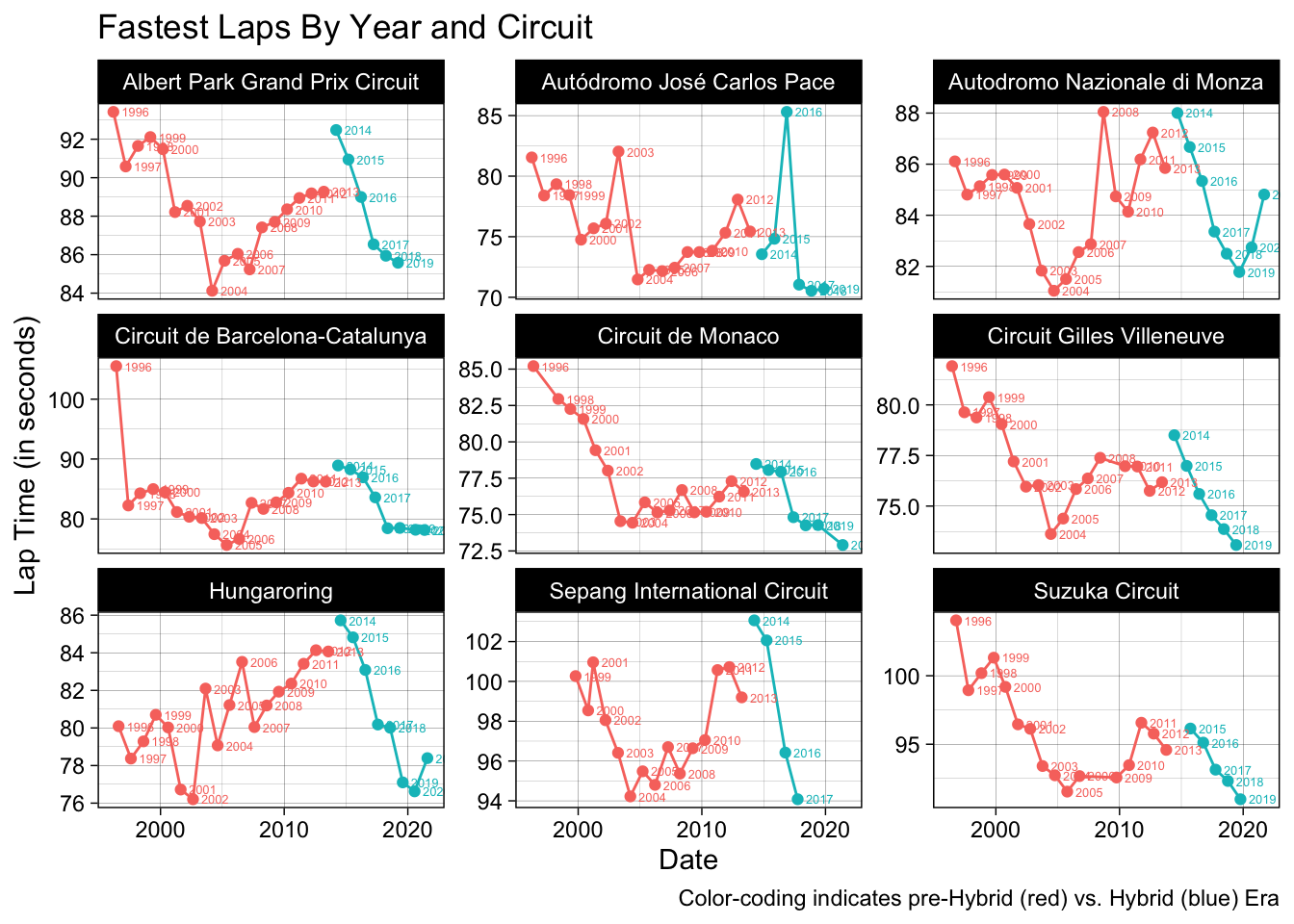
This visualization is a simple scatterplot superimposed with a time-series line graph, color-coded by pre-Hybrid vs Hybrid Era. First, it should be clarified that certain outliers are present that should not be considered in interpreting the data. Extremely high lap times, like those observed in Barcelona in 1996 or at Interlagos in 2016, correspond with wet-weather races, which tend to be significantly slower for obvious safety reasons. Certain years’ observations have been excluded entirely in the process of filtering out some of these outlier laps.
Once wet-weather laps are ignored, there is a distinct trend that emerges in these fastest lap data. Across almost all nine circuits, there is an observable increase in fastest lap time from 2013 to 2014, as well as a subsequent year-over-year decrease in fastest lap time across all circuits as the Hybrid Era progressed. In the case of every circuit (except Monza, arguably), the fastest lap of the most recent Grand Prix is significantly faster than that of the last pre-Hybrid Era Grand Prix. The general trend appears to be that, after a brief adjustment period when the new rules were implemented, racers continually improved lap times throughout the Hybrid Era, achieving lap times that in every case bettered those to be expected at the end of the pre-Hybrid era. This is a strong initial sign that racing improved over the course of the Hybrid Era – more specifically, that technological and racing improvements were continually being made between 2014 and 2021.
Race Laps
My second exploratory visualization concerns the distribution of lap times by circuit and year.
# Ridgeline plot of lap time distributions by circuit and year

lap_times %>%
  mutate(hybrid=case_when(
    seas_year>=2014 ~ 1,
    T ~ 0
  )) %>%
  filter(time_lap_ms<=115000) %>%
  filter(seas_year %in% c(1996:2021)) %>%
  filter(circ_id %in% c(1,2,4,6,7,11,14,18,22)) %>%
  filter(race_id!=c(1046)) %>%
  ggplot(aes(x = as.numeric(time_lap),
             y = as.factor(seas_year),fill=as.factor(hybrid),alpha=0.5)) +
  geom_density_ridges() +
  theme_linedraw() +
  theme(axis.text = element_text(size = 6.5)) +
  facet_wrap(vars(circ_name),scales="free_x") +
  theme(legend.position = "none") +
  labs(
    title="Distribution of Race Lap Times by Year and Circuit",
    caption="Color-coding indicates pre-Hybrid (red) vs. Hybrid (blue) Era",
    x="Lap Time (in Seconds)",
    y="Season Year"
  )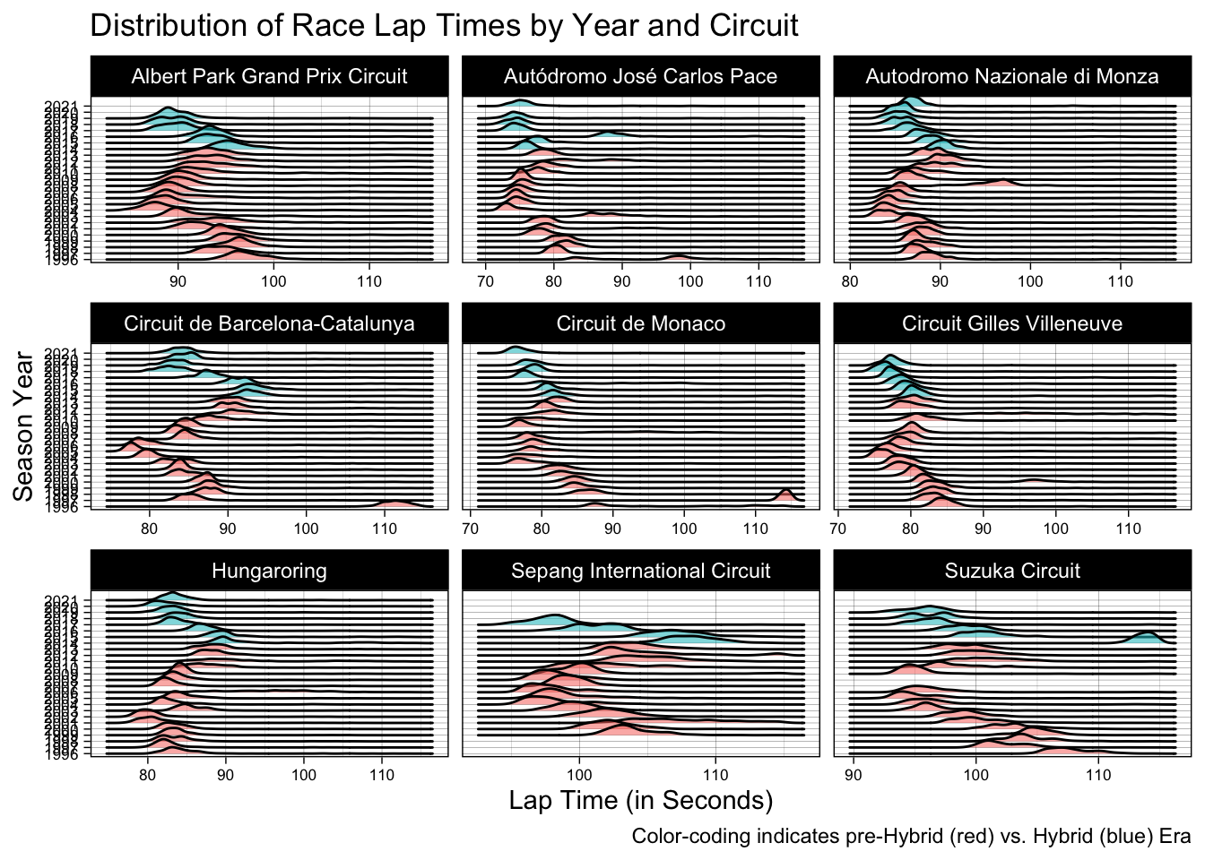
I chose to utilize a color-coded “ridgeline” plot for these distributions, allowing for simple year-by-year visual comparison. The individual “ridges” are density plots, reflecting the frequency (on the implied z-axis) of the given lap times on the x-axis, compared by year on the y-axis. Once again, color coding reflects whether a given year was pre-Hybrid Era (red) or Hybrid Era (blue).
Once again, there appears to be a year-over-year trend toward collectively faster lap times as the Hybrid Era progressed. Certain circuits, such as Sepang or Suzuka, saw a broad distribution of lap times, and can make for some difficult interpretation. However, other circuits like Monza, the Hungaroring, and especially Gilles Villeneuve show a much more concentrated distribution of lap times that trend toward an improvement over pre-Hybrid Era times. It should be noted that these are lap times from across the grid, rather than isolated fastest laps from single drivers. The concentration of lap times around these circuits suggests that racing remained competitive during the Hybrid Era, while the collective shift toward faster lap times illustrates improvements being made up and down the grid, and not only coming from certain constructors or drivers.
Qualifying Laps
My final visualization concerns qualifying times from across all three rounds of qualifying for Grands Prix held at the same nine circuits across the same 25-year period.
na.omit(qual_race) %>%
  filter(seas_year %in% c(1996:2021)) %>%
  filter(circ_id %in% c(1,2,4,6,7,11,14,18,22)) %>%
  filter(qual_time<ms("2:45.00")) %>%
  mutate(hybrid=case_when(
    seas_year>=2014 ~ 1,
    T ~ 0
  )) %>%
  ggplot(
    aes(x=as.numeric(qual_time),
        y=as.factor(seas_year),
        fill=as.factor(hybrid),alpha=0.5)
    ) +
  geom_density_ridges() +
  theme_linedraw() +
  theme(legend.position = "none") +
  facet_wrap(vars(circ_name),scales="free_x") +
  theme(axis.text = element_text(size = 6.5)) +
  labs(
    title="Distribution of Lap Times in Qualifying by Year and Circuit",
    caption="Color-coding indicates pre-Hybrid (red) vs. Hybrid (blue) Era",
    x="Lap Time (in Seconds)",
    y="Season Year"
  )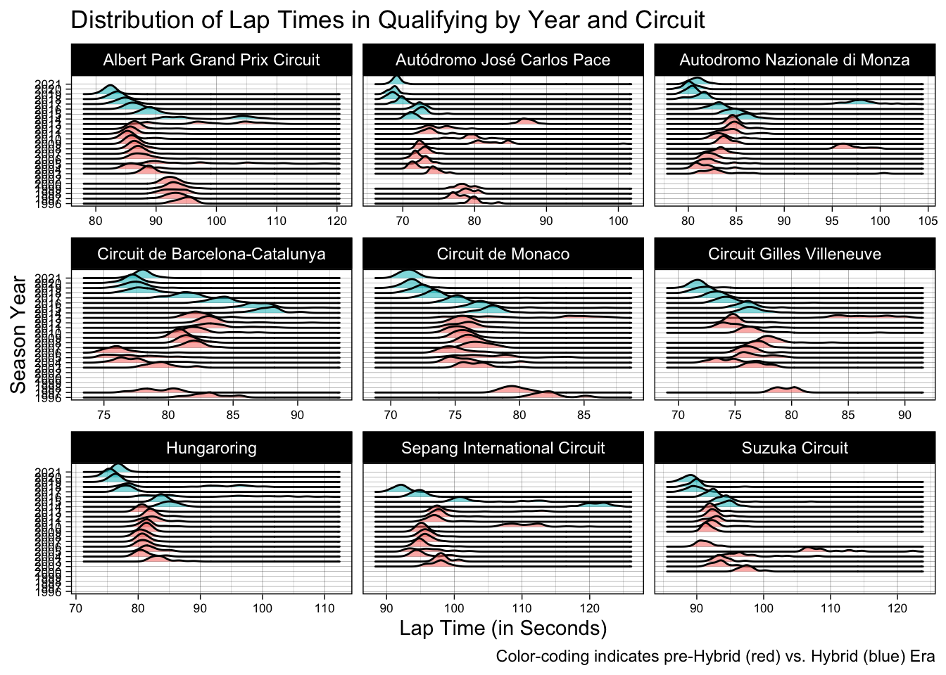
A similar ridgeline plot to the lap time visualization is used.
It is important to understand the mechanics of Formula 1 qualifying in order to properly interpret this plot. F1 qualifying sessions are not held as competitive races between cars, but rather as concurrent time-trials held over three rounds, the first two of which feature the elimination of the five slowest cars from that round. Only a driver’s best time from a given round is recorded, and the above plot amalgamates times across rounds for each year. It is also important to note that, traditionally, qualifying sessions are held on the day preceding the race, which can make for differing weather conditions. In general, then, the above plot reflects less upon wheel-to-wheel, on-track racing, and speaks more to the quality of the cars up and down the grid, particularly in terms of technological advancements.
Once again, this ridgeline plot illustrates an apparent trend toward year-over-year improvement, over and above the pre-Hybrid Era, across the grid throughout the duration of the Hybrid Era. This is perhaps most clearly seen in the Monaco circuit plot, with every Hybrid Era ridge (barring 2021) appearing to reflect a collective improvement on the previous race, which by 2016 are already faster than most or all of the qualifying time distributions from the pre-Hybrid Era. Additionally, these ridges once again remain concentrated throughout the Hybrid Era, suggesting that improvement was consistent across all constructors year over year.
Conclusion
This preliminary exploratory analysis of Formula 1 data from 1996 to 2021 suggests that racing consistently improved while remaining competitive throughout the duration of the sport’s Hybrid Era, especially when compared to data from seasons prior to this Era. Further analysis is needed, however, before conclusions can be drawn – analysis of overtaking data alongside lap time data, and analysis performed in a more statistically rigorous and scientific way.
Citations
“Ergast Developer API.” n.d. Ergast Developer API. Accessed September 3, 2022. http://ergast.com/mrd/.
FORMULA 1, dir. 2022. The End Of An F1 Era | 2014 To 2021. https://www.youtube.com/watch?v=T_55mVi_wQQ.
Grolemund, Garrett, and Hadley Wickham. 2017. R for Data Science. Sebastopol, CA: O’Reilly Media.
Vopani. n.d. “Formula 1 World Championship (1950 - 2022).” Accessed September 3, 2022. https://www.kaggle.com/datasets/rohanrao/formula-1-world-championship-1950-2020.
R Core Team (2022). R: A language and environment for statistical computing. R Foundation for Statistical Computing, Vienna, Austria. URL https://www.R-project.org/.
RStudio Team (2022). RStudio: Integrated Development Environment for R. RStudio, PBC, Boston, MA URL http://www.rstudio.com/.
Wickham H, Averick M, Bryan J, Chang W, McGowan LD, François R, Grolemund G, Hayes A, Henry L, Hester J, Kuhn M, Pedersen TL, Miller E, Bache SM, Müller K, Ooms J, Robinson D, Seidel DP, Spinu V, Takahashi K, Vaughan D, Wilke C, Woo K, Yutani H (2019). “Welcome to the tidyverse.” Journal of Open Source Software, 4(43), 1686. doi:10.21105/joss.01686 https://doi.org/10.21105/joss.01686.