---
title: "Final Project"
author: "Pavan Datta Abbineni "
desription: "Final Project"
date: "08/28/2022"
format:
html:
toc: true
code-fold: true
code-copy: true
code-tools: true
categories:
- Final Project
---
quarto-executable-code-5450563D
```r
#| label: setup
#| warning: false
#| message: false
library(tidyverse)
library(lubridate)
library(magrittr)
library(tidyverse)
library("viridis")
library(glue)
library(leaflet)
library(ggplot2)
library(plotrix)
library(lubridate)
library(scales)
library(plyr)
require(mosaic)
knitr::opts_chunk$set(echo = TRUE, warning=FALSE, message=FALSE)
```
### Introduction
According to the World Health Organization (WHO) stroke is the 2nd leading cause of death globally, responsible for approximately 11% of total deaths. This dataset is used to predict whether a patient is likely to get stroke based on the input parameters like gender, age, various diseases, and smoking status. Each row in the data provides relavant information about the patient.
### Dataset
#### About the Data
Data for this project originates from the Electronic Health Record (EHR) controlled by McKinsey & Company. This data is a well refined and filtered dataset of the original dataset which was collected over a course of several years in Bangladesh.
#### Project Goals
My main objective in this project is focused on finding the best lifestyle choices with the help of the attribute analysis in this dataset, inorder to prevent stroke.
#### Import the data
The HealthCareStrokeDataset is imported into R for cleaning, wrangling,exploration and analysis.
```{r readingData}
healthCareStrokeData<-read_csv("_data/healthcare-dataset-stroke-data.csv",
                        show_col_types = FALSE)
```
#### Attribute Information
* id (int, categorical): unique identifier
* gender (str, categorical): “Male”, “Female” or “Other”
* age (int, numerical): age of the patient
* hypertension (int, categorical): 0 if the patient doesn’t have hypertension, 1 if the patient has hypertension
* heart_disease (int, categorical): 0 if the patient doesn’t have any heart diseases, 1 if the patient has a heart disease
* ever_married (str, categorical): “No” or “Yes”
* work_type (str, categorical): “children”, “Govt_jov”, “Never_worked”, “Private” or “Self-employed”
* Residence_type (str, categorical): “Rural” or “Urban”
* avg_glucose_level (int, numerical): average glucose level in blood
* bmi (str, numerical): body mass index*
* smoking_status (str, categorical): “formerly smoked”, “never smoked”, “smokes” or “Unknown”*
* stroke (int, categorical): 1 if the patient had a stroke or 0 if not
Note: “Unknown, NA” in smoking_status and bmi means that the information is unavailable for this
patient
#### Tidy the data
To learn more about the dataset let's get an idea of the column names, data dimensions, statistical summary comprised of min,max,median,mean and interquartile range.
```{r dataSummary}
summary(healthCareStrokeData)
dim(healthCareStrokeData)
names(healthCareStrokeData)
```
To get a further insight into the dataset lets print in three different ways
* Head of the dataset,
* Tail of the dataset and
* Randomly print 'n' elements from the dataset.
```{r data-head}
head(healthCareStrokeData)
```
```{r data-tail}
tail(healthCareStrokeData)
```
```{r data-random}
randomlySelectedData <- healthCareStrokeData[sample(1:nrow(healthCareStrokeData), 5), ]
randomlySelectedData
```
We can see that each row in our dataset is a unique observation which represents a unique persons lifestyle and if they had a stroke or not.
Each variable is seen as one consistent data type, thus some variables are numeric and some are categorical. The datatype of each column is elaborated below.
* Categorical : Gender, Ever_married, Work_type, Residence_type, smoking_status
* Categorical ( Boolean ) : Hypertension, Heart_disease, stroke_label
* Quantitative (continuous) : avg_glucose_level, bmi
* Quantitative (discrete) : age
Let's check for any na values in our dataset.
```{r check-na}
sum(is.na(healthCareStrokeData))
```
Next lets check our dataset for any duplicate rows.
```{r checkForDuplicates}
nOccur <- data.frame(table(healthCareStrokeData$id))
nOccur[nOccur$Freq > 1,]
```
From the above result we can confirm that there are no duplicates in our dataset.
From the datatype of bmi we can see that it is in string format, we need to convert into numeric.
```{r convertBMI}
healthCareStrokeData$bmi <- as.numeric(healthCareStrokeData$bmi)
```
As we can see there are NA values introduced by coercion, so let's drop all the NA values before going to the next step.
```{r check-na_2}
sum(is.na(healthCareStrokeData))
```
```{r omit-na}
healthCareStrokeData <- na.omit(healthCareStrokeData)
```
As our main interest in this project are only the people who had a stroke lets filter our dataset to only contain who had a stroke.
```{r onlyStrokeData}
healthCareOnlyStroke <- healthCareStrokeData %>% filter(stroke == 1)
```
Let's do a , statistical summary comprised of min,max,median,mean and interquartile range,column names, data dimensions for our target dataset.
```{r dataSummary-targetData}
summary(healthCareOnlyStroke)
dim(healthCareOnlyStroke)
```
### Data Analysis and Visualization
Now that our dataset has been imported, cleaned, and tidied it can be used for further visualization and analysis. Let's begin our analysis with the most basic questions like the mean and median of our age, bmi and avg_glucose_level.
As stated above the main variables I'm going to focus on are :
* age
* bmi and
* avg_glucose_level
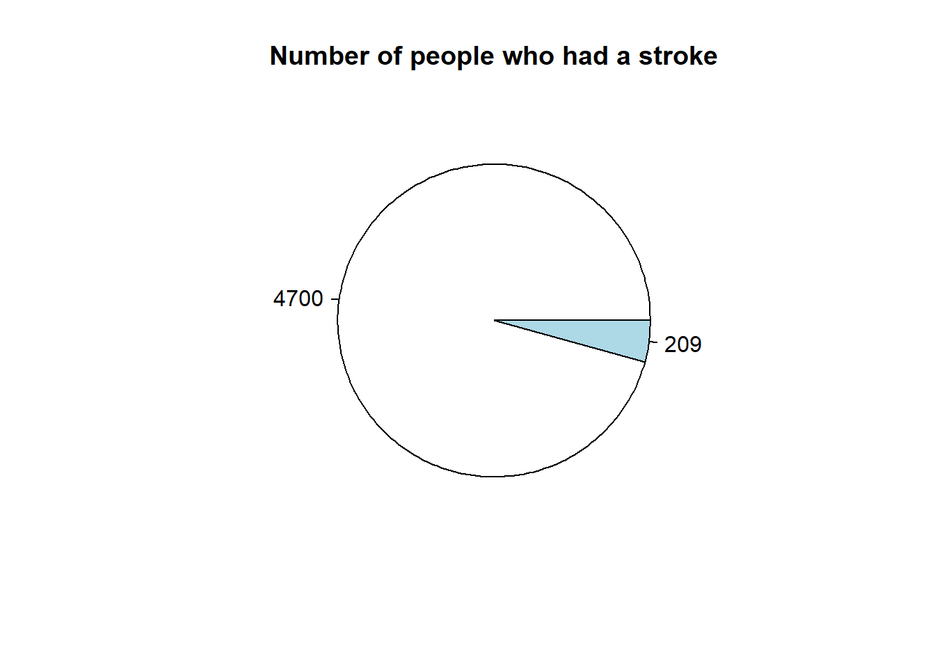
```{r stroke-piechart}
strokeLabels  = table(healthCareStrokeData$stroke)
pie(strokeLabels,labels = strokeLabels, main = "Number of people who had a stroke")
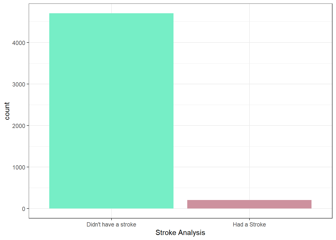
histogramStrokeData<-healthCareStrokeData
histogramStrokeData$stroke <- factor(histogramStrokeData$stroke,
                         levels = c(0,1),
                         labels = c("Didn't have a stroke","Had a Stroke"))
ggplot(histogramStrokeData, aes(stroke,))+
  geom_bar(fill=c("aquamarine2","pink3")) +
  theme_bw()+
  theme(plot.title = element_text(hjust = 0.5))+
  xlab("Stroke Analysis")
```
```{r stroke-stats}
favstats((healthCareStrokeData %>% filter(stroke == 0))$age)
```
```{r nostroke-stats}
favstats((healthCareStrokeData %>% filter(stroke == 1))$age)
```
#### Effect of Age
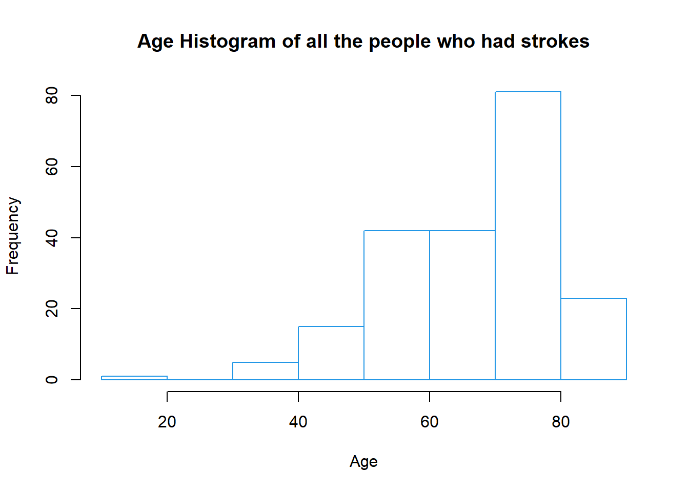
```{r strokeAge-histogram}
strokeAgeLabels<-(healthCareStrokeData %>% filter(stroke == 1))$age
hist(strokeAgeLabels,
     main = "Age Histogram of all the people who had strokes",
     xlab = "Age",
     col = "white",
     border = 4)
```
We can see that the risk of having a stroke is a lot higher in the 70-80 age bracket.But age is something we cannot overcome so let's have a detailed analysis of other attributes.
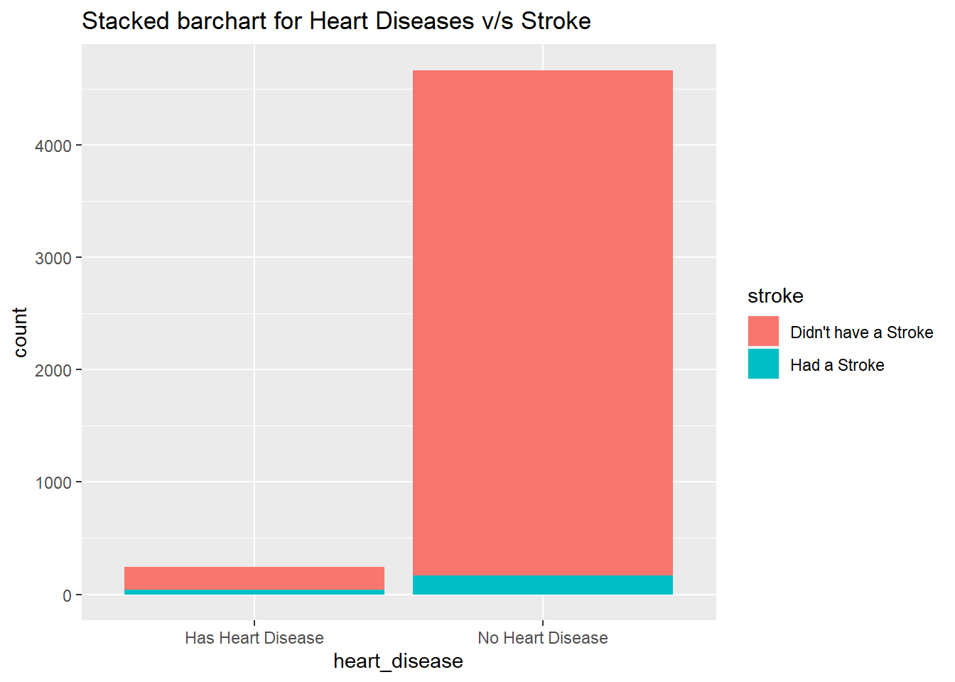
#### Effect of heart_disease
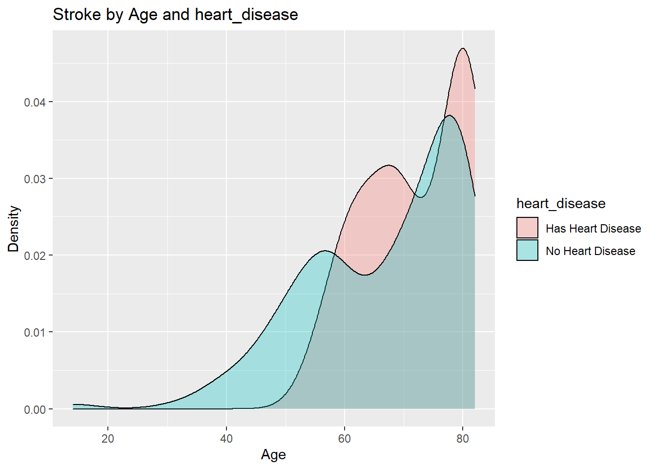
```{r heartDisease-ggplot}
datasetForHeartAnalysis<-healthCareStrokeData
datasetForHeartAnalysis$heart_disease[datasetForHeartAnalysis$heart_disease == 0]<-"No Heart Disease"
datasetForHeartAnalysis$heart_disease[datasetForHeartAnalysis$heart_disease == 1]<-"Has Heart Disease"
datasetForHeartAnalysis$stroke[healthCareStrokeData$stroke == 0]<-"Didn't have a Stroke"
datasetForHeartAnalysis$stroke[healthCareStrokeData$stroke == 1]<-"Had a Stroke"

datasetForHeartAnalysis %>% filter(stroke=="Had a Stroke")%>%
                        ggplot(aes(age, fill=heart_disease)) +
                        geom_density(alpha=0.3) +
                        ggtitle("Stroke by Age and heart_disease") +
                        xlab("Age") +
                        ylab("Density")
ggplot(data = datasetForHeartAnalysis,
       aes(x=heart_disease,
           fill=stroke,)) +
          geom_bar() +
          ggtitle("Stacked barchart for Heart Diseases v/s Stroke")
```
```{r heartdisease-cal}
tableDatasetForHeartAnalysis<-datasetForHeartAnalysis%>%filter(heart_disease=="Has Heart Disease")
table(tableDatasetForHeartAnalysis$stroke)
tableDatasetForHeartAnalysis<-datasetForHeartAnalysis%>%filter(heart_disease=="No Heart Disease")
table(tableDatasetForHeartAnalysis$stroke)
```
We have a 16% chance to have a stroke if you have a heart disease and a 3.6% chance to have a stroke if you don't have a heart disease.
From the above data/plots it is clearly evident that the people with heart diseases are more likely to have a stroke as they age.
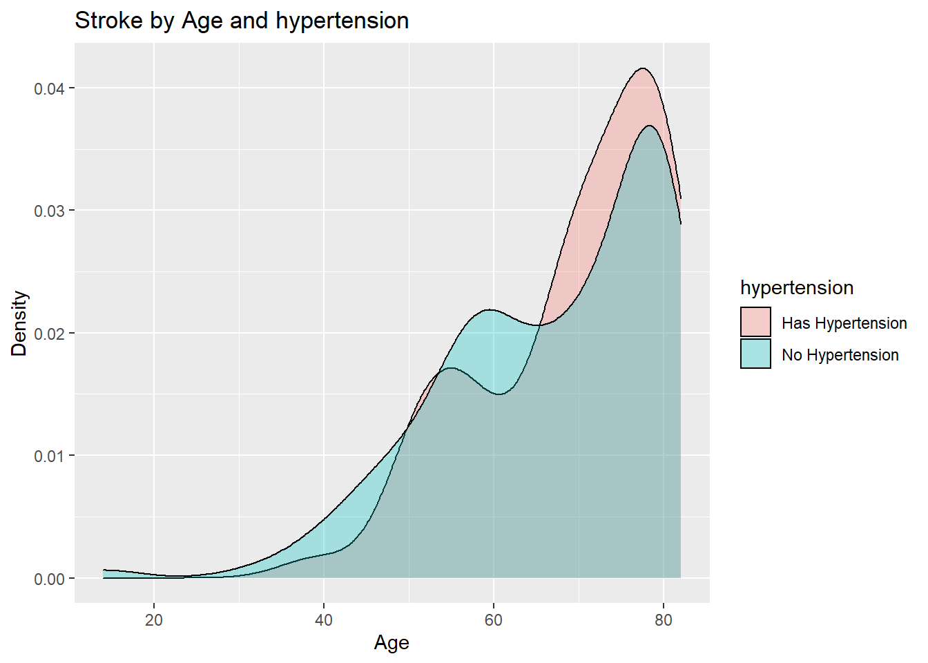
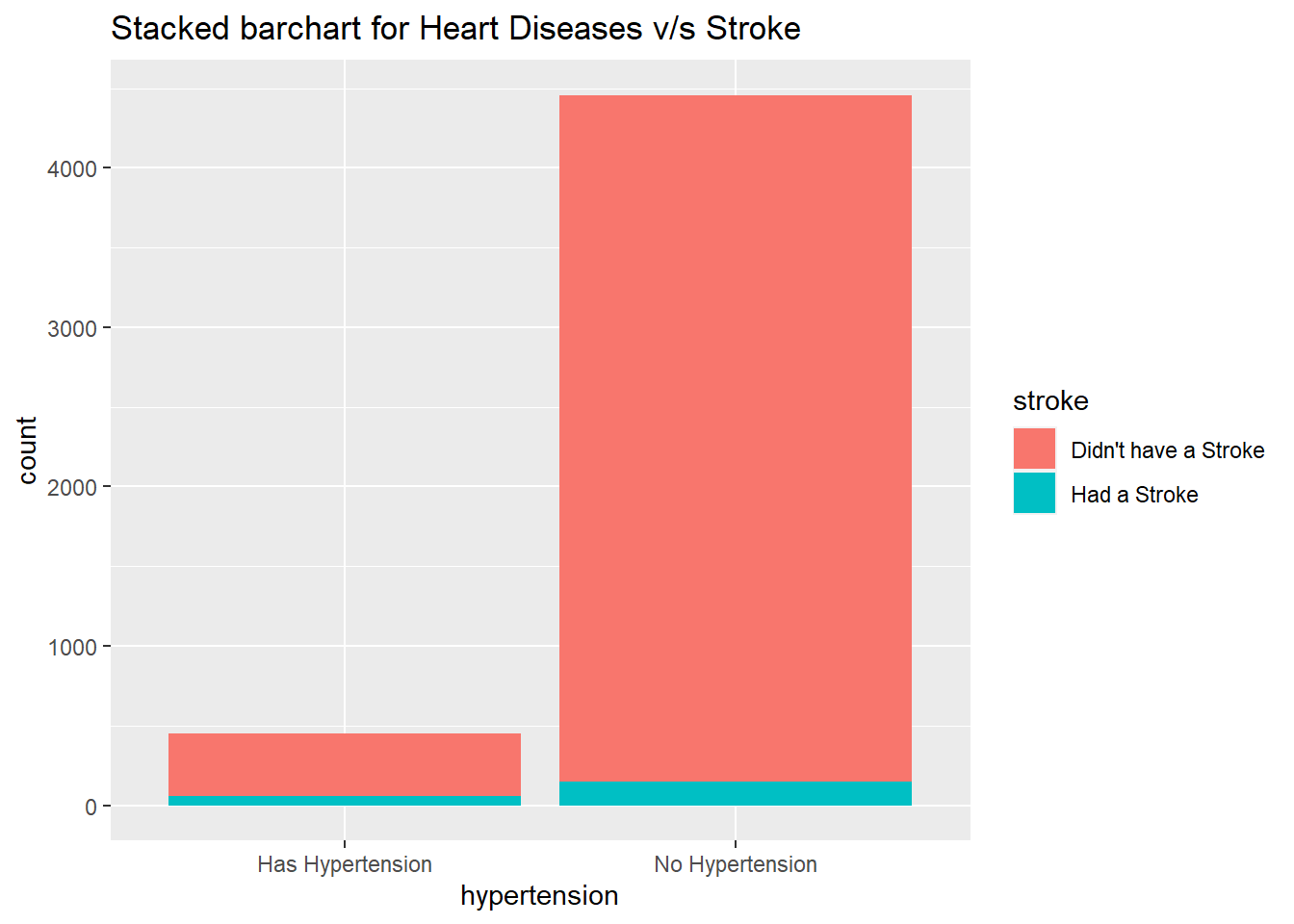
#### Effect of hypertension
```{r hypertension-ggplot}
datasetForHypertensionAnalysis<-healthCareStrokeData
datasetForHypertensionAnalysis$hypertension[datasetForHypertensionAnalysis$hypertension == 0]<-"No Hypertension"
datasetForHypertensionAnalysis$hypertension[datasetForHypertensionAnalysis$hypertension == 1]<-"Has Hypertension"
datasetForHypertensionAnalysis$stroke[datasetForHypertensionAnalysis$stroke == 0]<-"Didn't have a Stroke"
datasetForHypertensionAnalysis$stroke[datasetForHypertensionAnalysis$stroke == 1]<-"Had a Stroke"

datasetForHypertensionAnalysis %>% filter(stroke=="Had a Stroke")%>%
                        ggplot(aes(age, fill=hypertension)) +
                        geom_density(alpha=0.3) +
                        ggtitle("Stroke by Age and hypertension ") +
                        xlab("Age") +
                        ylab("Density")
ggplot(data = datasetForHypertensionAnalysis,
       aes(x=hypertension,
           fill=stroke,stat="count")) +
          geom_bar() +
          ggtitle("Stacked barchart for Heart Diseases v/s Stroke")
```
```{r hypertension-cal}
tableDatasetForHypertension<-datasetForHypertensionAnalysis%>%filter(hypertension=="Has Hypertension")
table(tableDatasetForHypertension$stroke)
tableDatasetForHypertension<-datasetForHypertensionAnalysis%>%filter(hypertension=="No Hypertension")
table(tableDatasetForHypertension$stroke)
```
We have a 13.33% chance to have a stroke if you have a heart disease and a 3.34% chance to have a stroke if you don't hypertension
We can see that we are at a higher chance ( approximately 4 times ) of having a stroke if you have hypertension.
What if a person has both hypertension and heart disease?
```{r dualanalysis-calc}
tableForDualAnalysis<-healthCareStrokeData%>%filter(hypertension==1 & heart_disease==1)
table(tableForDualAnalysis$stroke)
```
We can see that a person having both hypertension and heart disease has a 19% chance to have a stroke.
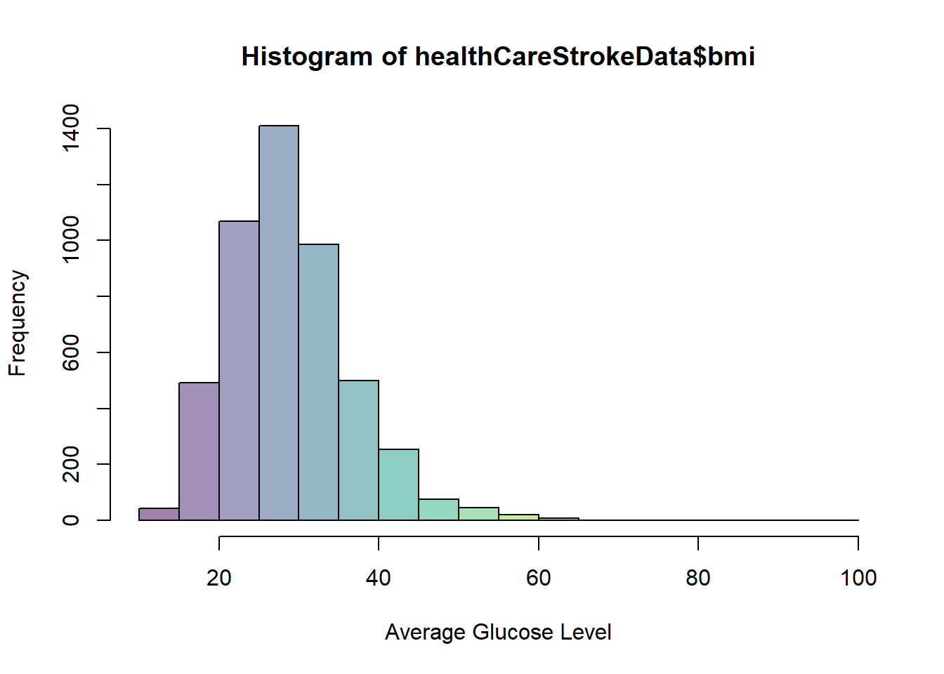
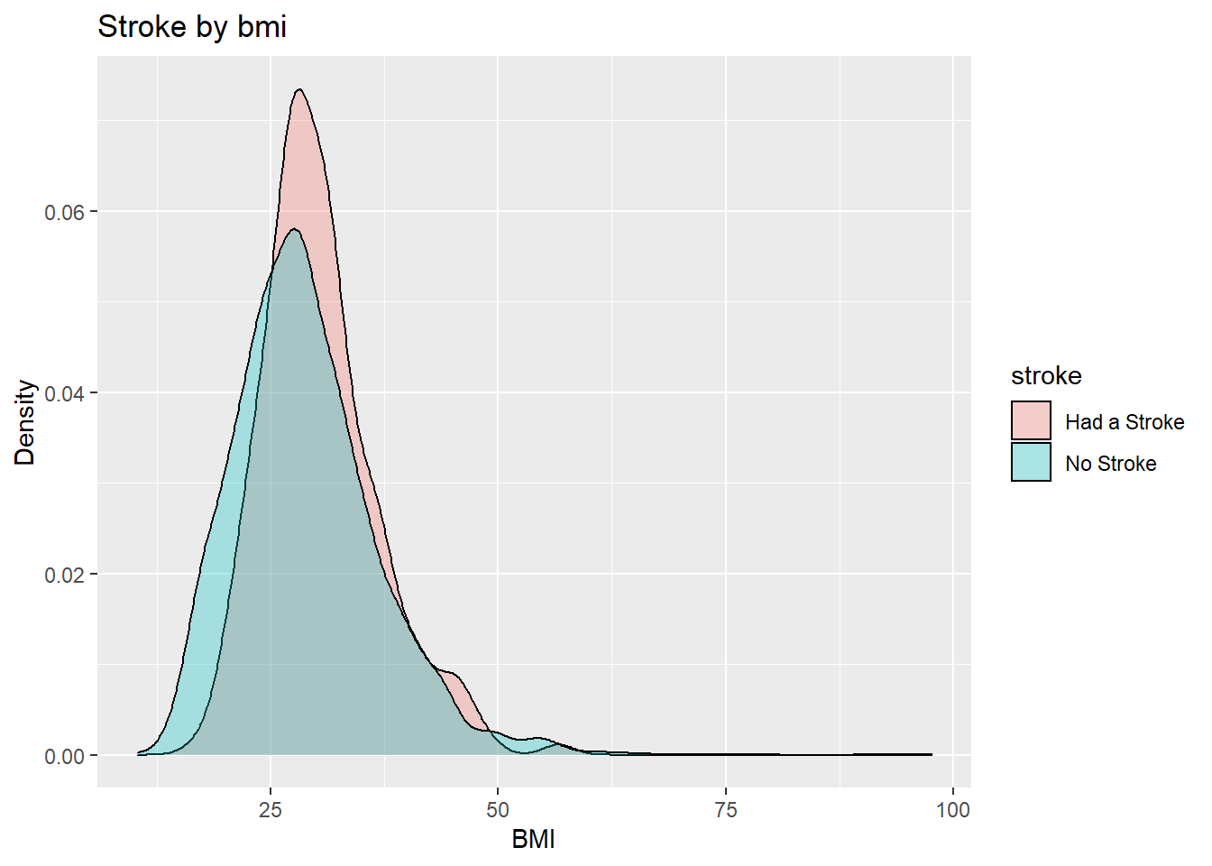
#### Effect of bmi
```{r bmi-ggplot}
hist(healthCareStrokeData$bmi,col=viridis(12,0.5),xlab = "Average Glucose Level")
datasetForbmiAnalysis<-healthCareStrokeData
datasetForbmiAnalysis$stroke[datasetForbmiAnalysis$stroke == 0]<-"No Stroke"
datasetForbmiAnalysis$stroke[datasetForbmiAnalysis$stroke == 1]<-"Had a Stroke"
datasetForbmiAnalysis %>% ggplot(aes(bmi, fill=stroke)) + geom_density(alpha=0.3) + ggtitle("Stroke by bmi") + xlab("BMI") + ylab("Density")
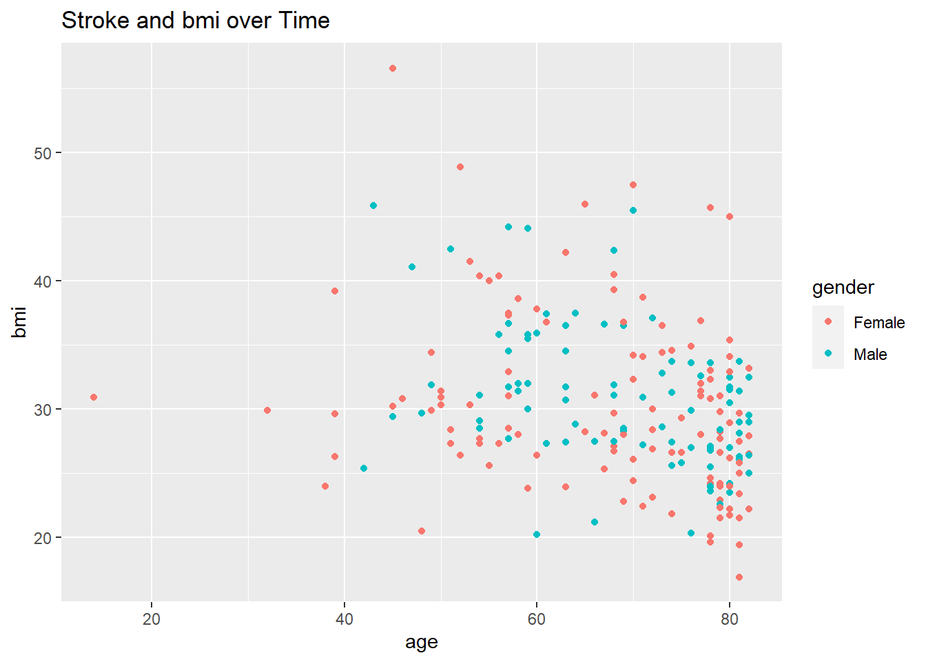
healthCareOnlyStroke %>% ggplot(aes(age, bmi, color=gender)) + geom_point() + ggtitle("Stroke and bmi over Time")
```
We can see that if you have a bmi greater than 25( overweight ) then you are more likely to have a stroke.
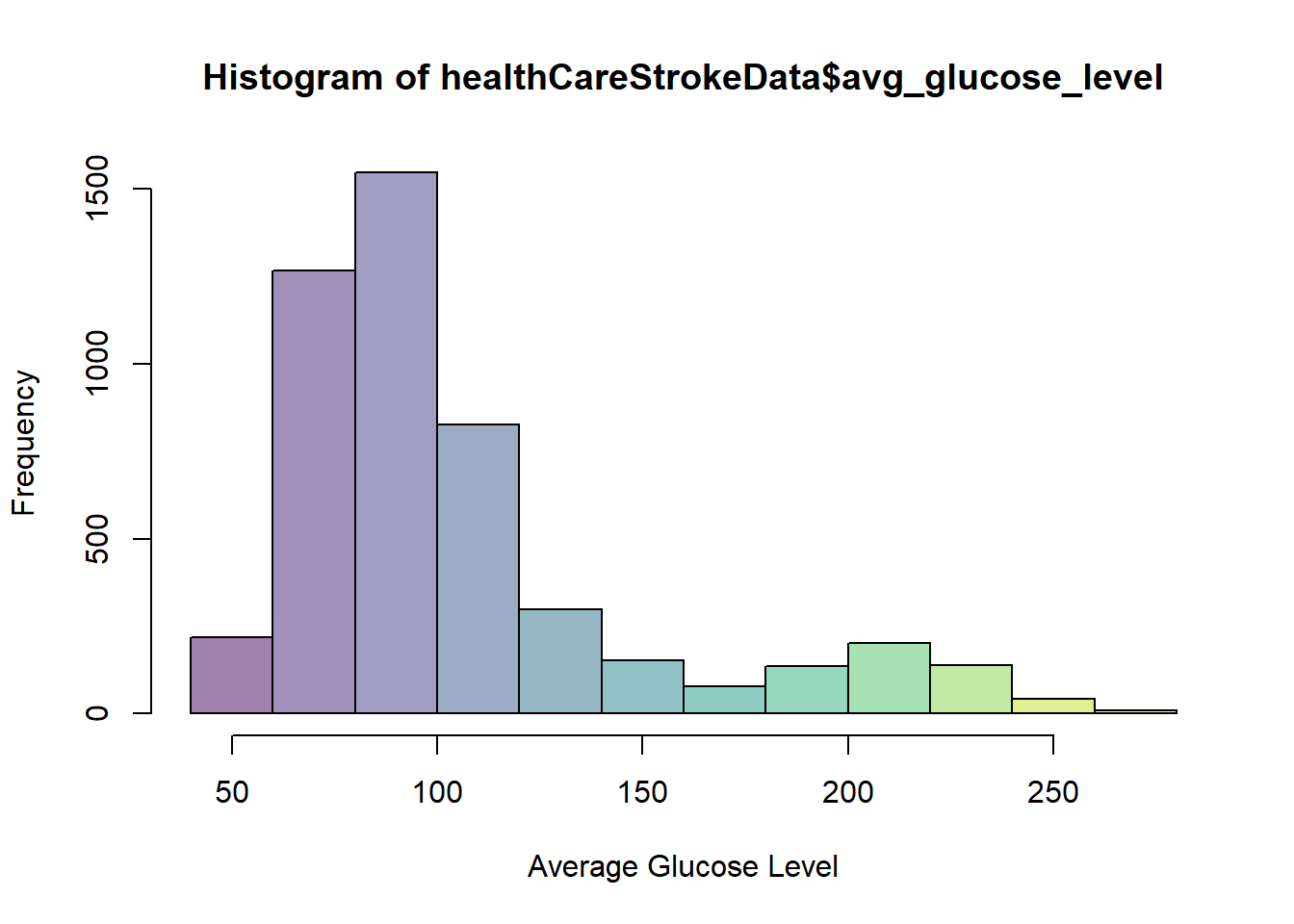
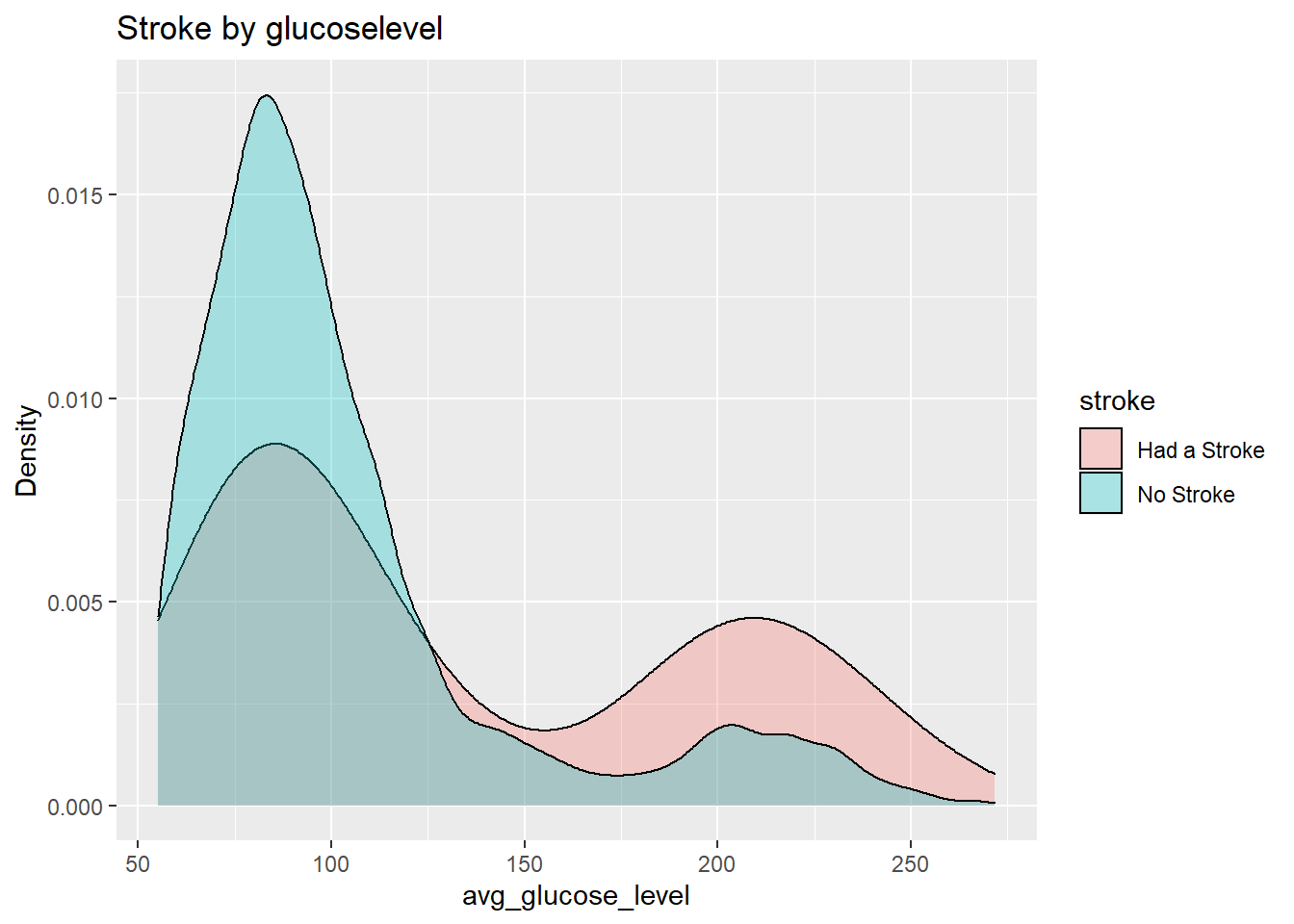
#### Effect of Glucose Level
```{r glucose-ggplot}
hist(healthCareStrokeData$avg_glucose_level,col=viridis(12,0.5),xlab = "Average Glucose Level")
datasetForGlucoseAnalysis<-healthCareStrokeData
datasetForGlucoseAnalysis$stroke[datasetForGlucoseAnalysis$stroke == 0]<-"No Stroke"
datasetForGlucoseAnalysis$stroke[datasetForGlucoseAnalysis$stroke == 1]<-"Had a Stroke"
datasetForGlucoseAnalysis %>% ggplot(aes(avg_glucose_level, fill=stroke)) + geom_density(alpha=0.3) + ggtitle("Stroke by glucoselevel") + xlab("avg_glucose_level") + ylab("Density")
```
Similar to the case of bmi the chances of having a stroke is higher at higher glucose levels.
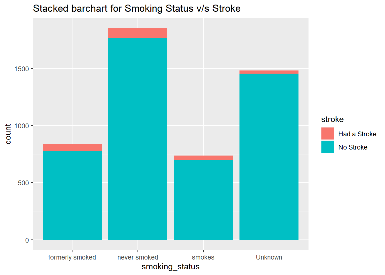
#### Effect of Smoking
```{r smoking-ggplot}
datasetForSmokingAnalysis<-healthCareStrokeData
datasetForSmokingAnalysis$stroke[datasetForSmokingAnalysis$stroke == 0]<-"No Stroke"
datasetForSmokingAnalysis$stroke[datasetForSmokingAnalysis$stroke == 1]<-"Had a Stroke"

ggplot(datasetForSmokingAnalysis,
       aes(x=smoking_status,
           fill=stroke,)) +
  geom_bar() + ggtitle("Stacked barchart for Smoking Status v/s Stroke")
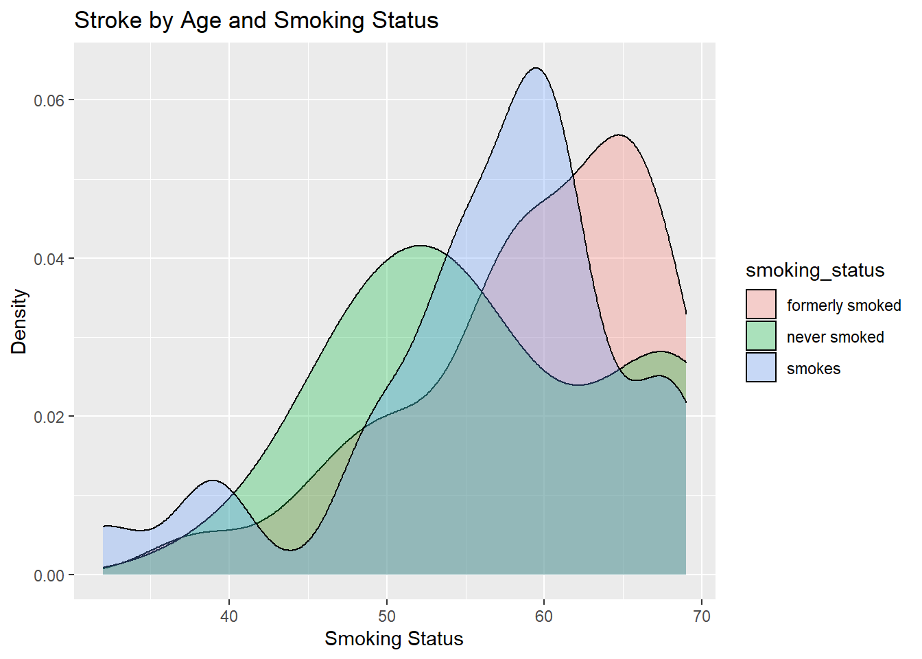
datasetForSmokingAnalysis %>%
  filter(stroke == "Had a Stroke" & age<70 &smoking_status!="Unknown")%>%
  ggplot(aes(age, fill=smoking_status)) +
  geom_density(alpha=0.3) +
  ggtitle("Stroke by Age and Smoking Status") +
  xlab("Smoking Status") + ylab("Density")
```
From the plot we can conclude that former smokers and a person who smokes is more likely to have a stroke when compared to a person who doesn't smoke.
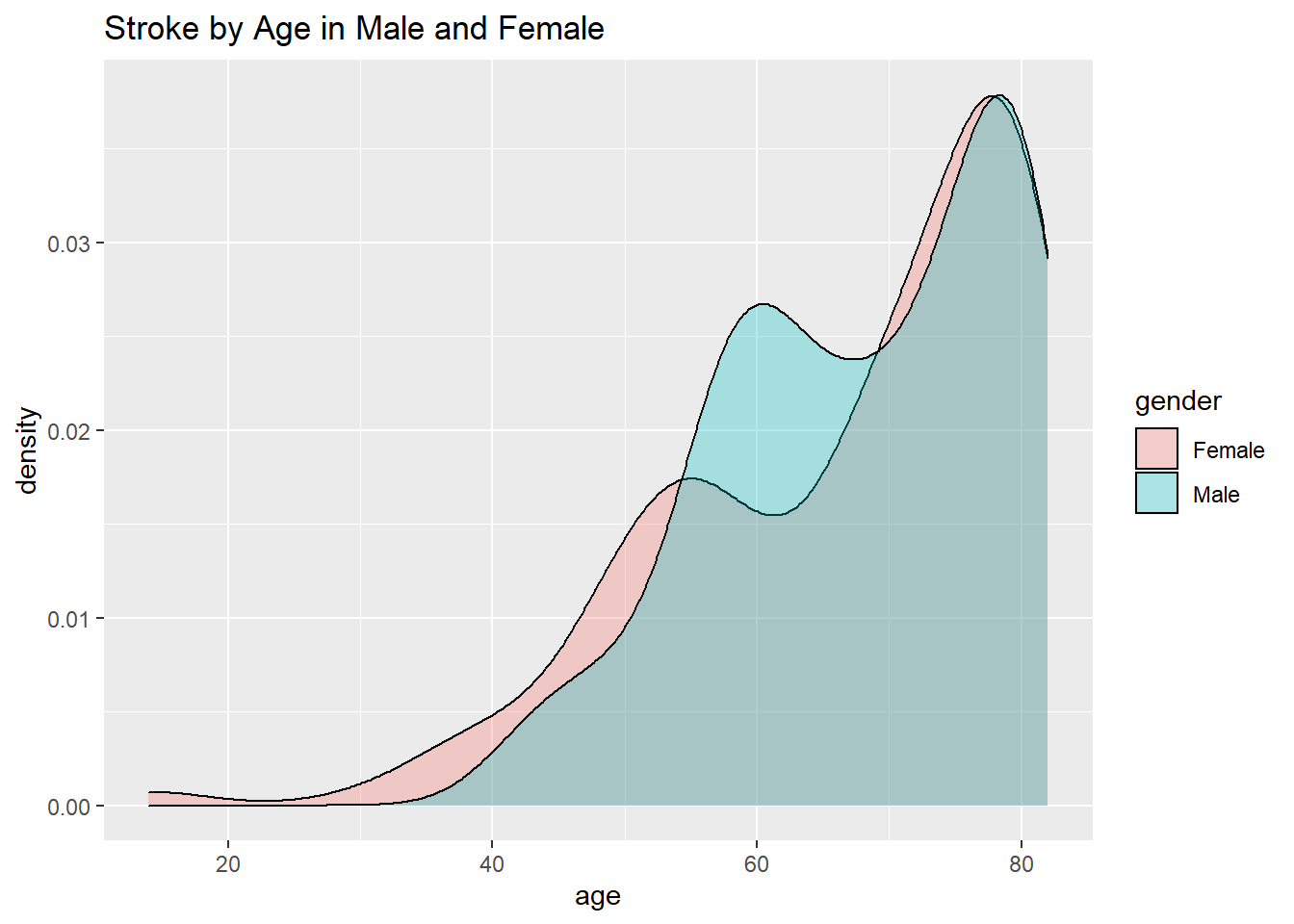
#### Effect of Gender
```{r gender-ggplot}
healthCareOnlyStroke %>% ggplot(aes(age, fill=gender)) + geom_density(alpha=0.3) + ggtitle("Stroke by Age in Male and Female")
```
We can see that as the age increases women tend to be prone to having a stroke at an earlier age while men develop it over time.
### Conclusion
Now that we have a detailed analysis of all the indicators that cause a stroke in our dataset, you can check for yourself how close you are to having a stroke. One thing we have no control over is age as everyone ages, but the rest of the attributes give us a lucid understanding of what to do to decrease our chances of having a stroke. A good start would be to quit smoking, Manage Stress, Normalize bmi, having low glucose level and having a better heart health.
I hope this study helps you make a data-driven decision about your health and lifestyle in order to prevent strokes.
### Bibliography/ References
[1] https://ieeexplore.ieee.org/stamp/stamp.jsp?arnumber=9264165
[2] https://ggplot2.tidyverse.org
[3] https://r-graph-gallery.com/stacked-barplot.html
[4] https://education.rstudio.com/learn/beginner/