Code
library(tidyverse)
knitr::opts_chunk$set(echo = TRUE, warning=FALSE, message=FALSE)library(tidyverse)
knitr::opts_chunk$set(echo = TRUE, warning=FALSE, message=FALSE)For my final project, I’m interested in working with data from Formula 1 (the motorsport racing series).
Formula 1 (F1) is the top class of single-seater motorsport racing. “Formula” refers to the set of rules to which all participants’ cars must conform. For example, Formula 2 has different rules about car design and racing than Formula 1.
An F1 season consists of a series of races, known as Grands Prix (GP), which take place around the world on purpose-built racing circuits as well as public roads (termed “street circuits”). The number and location of races per season has varied significantly across the years.
There are currently 10 teams in Formula 1, officially termed “Constructors”. Like the races, the number of teams (and names) has varied significantly over time. Each team has two drivers who race for them each season (as well as a driver on standby in case one of the primary drivers get sick/injured).
Each Constructor is responsible for designing their own car each season within a shared set of regulations that restrict the design across all teams (e.g. a minimum weight, certain aerodynamic requirements, etc.). Some Constructors are known as “works teams”. These teams design and construct the engines for their cars in addition to the aerodynamic components. The rest of the teams are called “customer teams”. They design the aerodynamic parts of their car, but purchase their engines from one of the works teams instead of designing it themselves. For example, currently, the Mercedes works team uses their engines for their own car and also provides engines to the Williams and McLaren teams.
There is also the concept of “junior teams”, where one company essentially has ownership over multiple teams in F1. They have one primary, A-team, and then a B-team that they can use to develop talent for their A-team. For example, currently Red Bull owns both the Red Bull Racing and Alpha Tauri teams, and regularly promote their drivers from Alpha Tauri to Red Bull Racing. For the purposes of the championship, however, these are considered separate constructors.
Because each Constructor designs their own car, cars can vary quite dramatically across teams, so there tends to be a somewhat clear hierarchy. The “worst” car often has nearly zero chance of winning a race, and the “best” cars almost always end up on the podium. In formula 1 lingo, teams are broken into three categories:
Due to this team hierarchy, it can be difficult to compare a driver from one team to a driver on another. Just because one driver always has faster lap times or finishes in a better position does not mean that they are necessarily a better driver, and could just mean that they have a better car. Since both teammates on a given team drive the same car, driver skill is often judged more-so based on how well a driver does compared to their teammates.
In each season, there are two separate championships up for grabs – a Drivers Championship and a Constructors Championship. The Drivers Championship is considered more prestigious and awards the individual driver who received the most points throughout the season. The Constructors Championship is awarded to the team with the most combined points across their two drivers.
Teams and drivers have the chance to earn points at each Grand Prix (note that there are also points available in what are called “Sprint races”, but these are a new feature in F1 and we’ll be excluding them for the purposes of this analysis in order to simplify things).
Each GP occurs over one weekend is broken up into two segments: qualifying (typically on Saturday) and the race (typically on Sunday). In qualifying, drivers try to put together the fastest lap. Lap times then determine the order that the cars will start for the race.
Within the race, cars are required to make at least one pit stop to change which type of tires they are using (there are hard, medium, and soft tires available for each race, each of which have different pros and cons). Depending on how much a given track damages the tires, along with other factors such as if a car is involved in a collision, additional pitstops may take place to change tires or swap out parts.
At the end of the race, points are awarded based on drivers’ finishing position. Additionally, the driver who records the fastest single lap throughout the race is awarded an extra point in addition to their points for finishing position.
The current points distribution is as follows:
Points are cumulative across a season, and the championships are awarded to the team and driver with the highest point totals.
The dataset I’ll be using is hosted on Kaggle at the following link: https://www.kaggle.com/datasets/rohanrao/formula-1-world-championship-1950-2020
It contains F1 race data from the series’ start in 1950 to the present season, which is currently in-progress and will run until November.
There are 14 separate files within this dataset:
circuits.csv contains information about the different tracks the drivers race on (a row here is a track)constructor_standings.csv contains information about how many points each team has after each race (a row here is a single team at a single race)constructors.csv stores the names and nationalities of teams (a row here is a team)driver_standings.csv stores information about how many points each driver was awarded at each race (a row here is a single driver at a single race)drivers.csv stores the names and nationalities of drivers (a row here is a driver)lap_times.csv stores the lap times for every driver on every lap of each race (a row here is a single lap for a single driver at a single race)pit_stops.csv stores information about every pit stop taken during each race (a row here is a single pit stop taken by a single driver at a single race)qualifying.csv stores qualifying lap times for each driver from each GP (a row here is a single driver in a single GP, and each row contains all qualifying lap times across multiple sessions)races.csv contains information about each GP, e.g. track name, date, etc. (a row here is a single GP)results.csv contains all of the finishing results for each race, e.g. driver finishing positions, # laps completed, fastest lap (a row here is a single driver at a single race)seasons.csv contains the years and urls for wikipedia pages associated with each season (a row here is a season)sprint_results.csv same as results.csv but for sprint races, which we’ll be excluding (a row here is a single sprint race)status.csv contains the encodings of a status variable that is referenced in the results files (a row here is a status)We now look at each of these one by one, excluding the sprint race results.
circuits.csvcircuits <- readr::read_csv("_data/formula1/circuits.csv")head(circuits)Each circuit has a circuitId that uniquely identifies it. We also have location information. The column alt is not entirely clear, so we can remove it.
All of the data types seem reasonable here so there is no need to modify them. However, we have a bunch of data frames that are all going to have a column called name as we’ll see later. We should rename these columns to avoid confusion when we join tables in the future.
circuits <- circuits %>%
rename(circuit_name = name) %>%
select(-alt)
circuits %>% head(1)constructor_standings.csvconstructor_standings <- readr::read_csv("_data/formula1/constructor_standings.csv")head(constructor_standings)The constructors standings data has a unique identifier for each row, as well as an id that refers to the races df as well as the constructors df. For each constructor/race we see how many points they have after that race, their current standing in the championship, as well as their running tally of wins in the season so far.
All of the data types seem reasonable here as well. constructorId would make more sense as a factor, but we would want to wait until later on when we join tables together to make this update since this refers to a column in another table. For now, positionText seems to duplicate position so we can remove positionText.
constructor_standings <- constructor_standings %>%
select(-positionText)
constructor_standingsconstructors.csvconstructors <- readr::read_csv("_data/formula1/constructors.csv")constructorsFor each constructor we have a unique constructorId (211 of them), which can be used to join this data with other tables. We also get names, nationalities and wikipedia URLs.
All of the data types are reasonable here. Converting team names to factors would again be better after completing joins.
We can again rename the name column to avoid confusion later.
constructors <- constructors %>%
rename(constructor_name = name)
colnames(constructors)[1] "constructorId" "constructorRef" "constructor_name" "nationality"
[5] "url" driver_standings.csvdriver_standings <- readr::read_csv("_data/formula1/driver_standings.csv")driver_standingsThis file has the exact same format as the constructors standings. A unique ID for each row, a race ID and driver ID to join with other tables, cumulative points, race position, and a running count of wins.
Again, positionText duplicates position so we can remove it.
driver_standings <- driver_standings %>%
select(- positionText)
driver_standingsdrivers.csvdrivers <- readr::read_csv("_data/formula1/drivers.csv")driversWe have 857 unique drivers. Each driver has a unique ID, a race number, a 3 letter code used to refer to them on score sheets/race documentation, a full name, DOB, nationality, and wikipedia link.
Driver number seems like it should be numeric, but it makes sense to leave as a character because the numbers aren’t actually ordered in any way (drivers choose them based on personal preference). There does seem to be a strange missing data marker (\\N), so we will replace this with a normal NA.
drivers <- drivers %>%
mutate(number = na_if(number, "\\N"))
driversWe can look at the popularity of different nationalities to get a sense of the driver makeup of the sport. We see that British and American drivers have historically made up the vast majority, followed by drivers from Brazil and Argentina.
drivers %>%
group_by(nationality) %>%
summarize(n = n()) %>%
head(10) %>%
ggplot(aes(x = reorder(nationality, n), y = n)) + geom_col() + coord_flip() + xlab("Count") + ylab("Driver Nationality") + ggtitle("Top 10 Driver Nationalities 2015-present") + theme_minimal()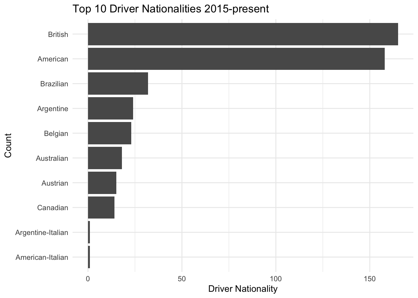
lap_times.csvlap_times <- readr::read_csv("_data/formula1/lap_times.csv")lap_timesLap times has unique identifiers referring to the race and driver who completed them, which we can use to join tables later. We also have lap number, driver position, and lap times. The time variable is in an hms class format, but to make analysis easier, we’ll get rid of it and just use the milliseconds column converted to seconds.
lap_times <- lap_times %>%
mutate(laptime_seconds = milliseconds/1000) %>%
select(-c(time, milliseconds))
lap_timesWe can look at the distribution of laptime_seconds with a histogram:
lap_times %>%
filter(laptime_seconds < 300) %>%
ggplot(aes(x=laptime_seconds)) + geom_histogram() + xlab("Lap Time in Seconds") + ylab("Count") + ggtitle("Distribution of Lap Times, 1950-present") + theme_minimal()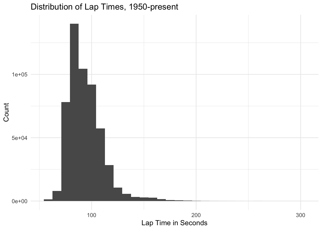
We can also generate a quick graph of how laptimes have changed from the first to the last recorded race in the data:
lap_times %>%
group_by(raceId) %>%
summarize(avg_lap = mean(laptime_seconds)) %>%
ggplot(aes(x= raceId, y=avg_lap)) + geom_point() + xlab("Race ID") + ylab("Avg Lap Time in Seconds") + ggtitle("Avg Lap Times From 1950-present") + theme_minimal()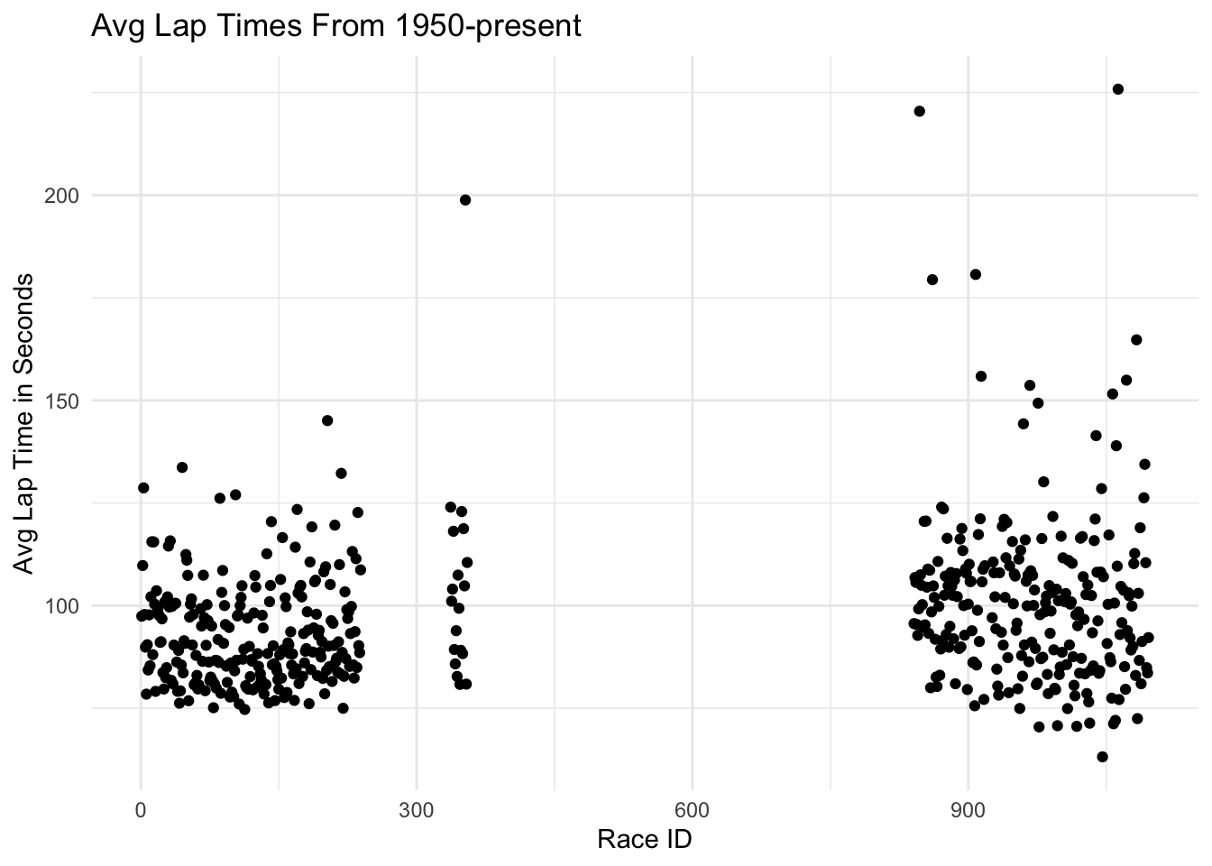
There seems to be a huge chunk of missing data in the middle. In the more recent races, lap times seem to have potentially decreased over time (though more analysis would be needed to determine this).
pit_stops.csvpit_stops <- readr::read_csv("_data/formula1/pit_stops.csv")pit_stopsFor the pit stops, we have a unique race and driver ID to join with other tables. We also get the stop number for that driver within the race, the lap in which the stop was taken, time of day and pit stop duration.
The only column with obviously the wrong data type is duration. Since this measures time, it should be a double. We can also rename duration to duration_seconds to make the units more obvious.
pit_stops <- pit_stops %>%
mutate(duration = as.numeric(duration)) %>%
rename(duration_seconds = duration)
pit_stopsLike lap times, we can look at the distribution of pit stop durations:
pit_stops %>%
filter(duration_seconds < 300) %>%
ggplot(aes(x=duration_seconds)) + geom_histogram() + xlab("Pit Stop Duration in Seconds") + ylab("Count") + ggtitle("Distribution of Pit Stop Durations, 1950-present") + theme_minimal()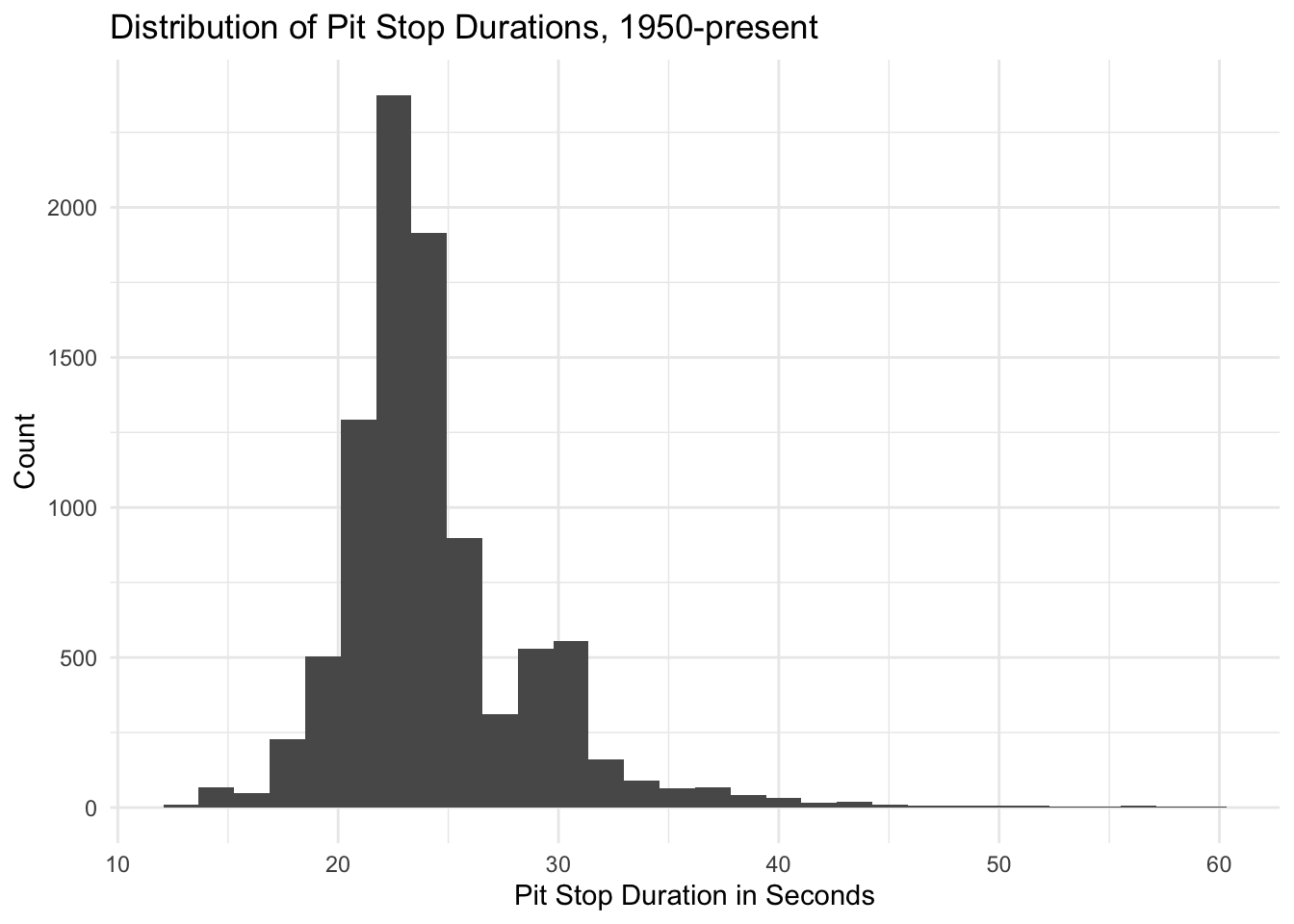
qualifying.csvqualifying <- readr::read_csv("_data/formula1/qualifying.csv")qualifyingFor qualifying, we get a unique race, driver, and constructor ID. We also have a column called “number” which is not entirely clear what it refers to. We then have overall qualifying position and qualifying times in the three different sections of qualifying (q1/q2/q3).
Since number is not clear, we can remove it. q1/q2/q3 are all times and should be converted as such. To make this easy, we’ll just convert the times to seconds. We’ll then rename the columns slightly to make them more clear. In the process, we’ll also replace the weird NA characters with normal NA values.
qualifying <- qualifying %>%
select(-number) %>%
mutate(across(q1:q3, ~ period_to_seconds(ms(na_if(.x, "\\N"))))) %>%
rename(q1_time_s = q1, q2_time_s = q2, q3_time_s = q3)
qualifyingWe can look at how times compare across each qualifying session:
qualifying %>%
select(contains("time_s")) %>%
rename(q1 = q1_time_s, q2 = q2_time_s, q3 = q3_time_s) %>%
pivot_longer(everything(), names_to = "session", values_to = "time_s") %>%
group_by(session) %>%
summarize(mean_time = mean(time_s, na.rm=TRUE), sd_time = sd(time_s, na.rm=TRUE))At a quick glance, we see that times seem to, on average, decrease from Q1 -> Q3. There is also more variability in Q1 than in the other sessions (which makes logical sense, as Q1 is the session that includes ALL cars, including those that are very slow/not fast enough to move on to Q2/Q3).
races.csvraces <- readr::read_csv("_data/formula1/races.csv")racesThis table contains information about each race – year, round (race number within year), circuit, race name, date, time, url, and some blank columns. For the purpose of analyzing anything about the sport, race dates and times are not relevant, so we’ll remove them. We can also remove all of the blank columns.
Again, we see the name variable, so we’ll rename this as well.
races <- races %>%
select(raceId:name) %>%
rename(gp_name = name)
racesresults.csvresults <- readr::read_csv("_data/formula1/results.csv")resultsFor race results, we see a race, driver, and constructor ID we can use to join other tables with. Again, we see a column called number that we don’t know what it means, so we can remove it.
grid represents starting position, so we can rename it as such (start_position).
For position, we have three different columns that are telling us something similar (almost duplicates). positionText is helpful because it shows us information such as whether the driver was disqualified (“D”) or whether they retired from the race (“R”). positionOrder is also helpful as this is the official classification used by F1 (D/R don’t matter for the classification). Rather than keep both positionText and positionOrder, we’ll keep positionOrder and then create new indicator columns for retirements and disqualifications. We will also rename position_order to finish_position to be more accurate.
The character representations of time are useless for analysis, so we’ll just keep milliseconds but convert to seconds. We will also make this a numeric column instead of character.
Fastest lap and rank should also be numeric, as should fastest lap speed. Fastest lap time should be converted to seconds like we did before.
Status ID is fine as is.
We make all of these modifications below:
results <- results %>%
mutate(
disqualified = as_factor(ifelse(positionText == "D", 1, 0)),
retired = as_factor(ifelse(positionText == "R", 1, 0)),
fastestLap = as.numeric(fastestLap),
rank = as.numeric(rank),
fastestLapTime = period_to_seconds(ms(na_if(fastestLapTime, "\\N"))),
fastestLapSpeed = as.numeric(fastestLapSpeed),
finishTimeSeconds = as.numeric(na_if(milliseconds, "\\N"))/1000) %>%
rename(start_position = grid, finish_position = positionOrder) %>%
select(-c(number, position, positionText, time, milliseconds))
resultsTo check our new variables, we can take a quick look at how number of disqualifications and retirements has changed over time.
results %>%
mutate(finished = as_factor(ifelse(statusId == 1, 1, 0))) %>%
select(raceId, disqualified, retired, finished) %>%
pivot_longer(disqualified:finished, names_to = "status", values_to = "status_met") %>%
filter(status_met == 1) %>%
group_by(raceId, status) %>%
summarize(count = n()) %>%
ggplot(aes(x=raceId, y=count, color=status)) + geom_smooth()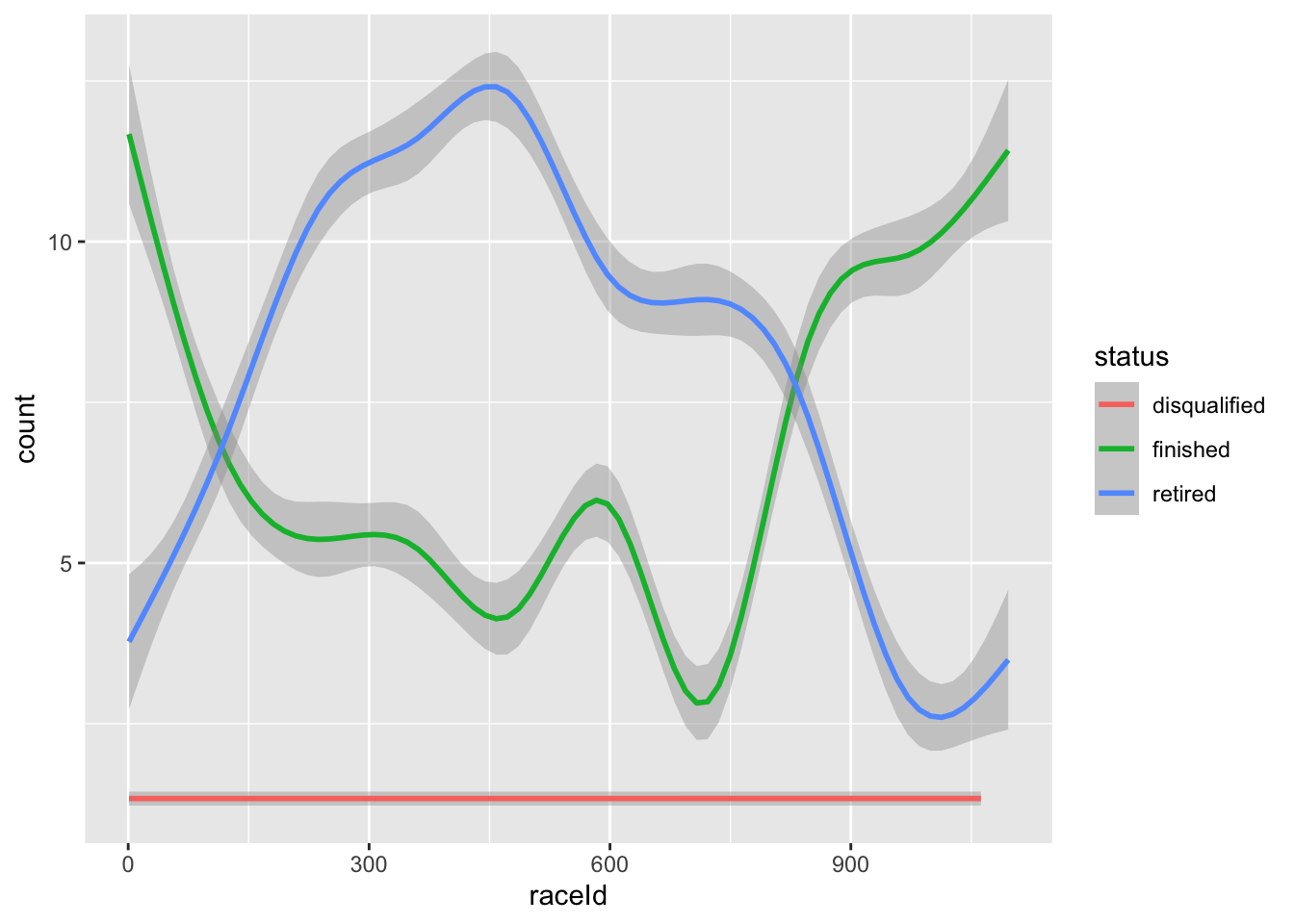
Using smoothing (so we don’t see too much noise), we see that disqualifications have remained steady and very low over time, while retirements and finishes have changed significantly, with a significant period where more cars retired than finished on average.
seasons.csvseasons <- readr::read_csv("_data/formula1/seasons.csv")seasonsThe seasons data is very simple and just has a year and wikipedia URL. There is no need to modify anything here, and this data overall does not look very useful.
status.csvstatus <- readr::read_csv("_data/formula1/status.csv")statusIn the results data frame there is a column called status ID:
results %>%
select(resultId, raceId, driverId, constructorId, start_position, finish_position, statusId)The status table contains the encodings for this table. For example, the first 5 status IDs are all 1, which indicates “Finished”, while the two people with status 5 had “Engine” issues.
We can quickly see what the top statuses are:
top_statuses <- results %>%
inner_join(status,by="statusId") %>%
group_by(statusId, status) %>%
summarize(n = n()) %>%
arrange(desc(n)) top_statuses %>%
head(15) %>%
ggplot(aes(x=reorder(status,n), y=n)) + geom_col() +
ggtitle("Most Common Race Statuses by Count") + theme_minimal() + xlab("Status") + ylab("Count") + coord_flip()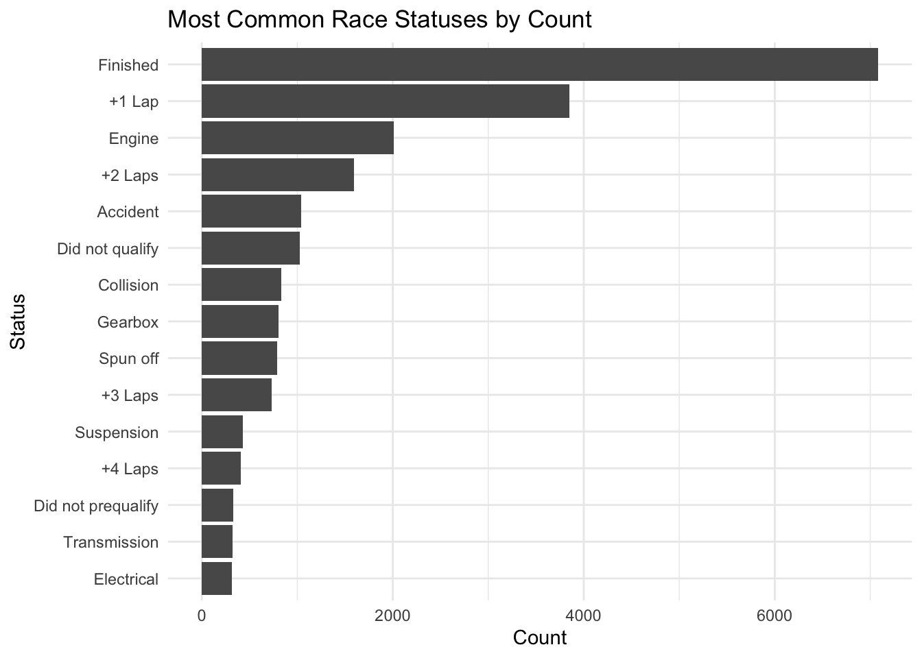
Most drivers finished. A good number were lapped. Most common reasons for DNF appear to be engine failure, accident, and collision.
As we can see, the status table will only be useful if joined with the results table in future analysis.
We don’t need to change anything about the data types in the status table. They all look good.
In 2022, there was a big regulations change that shifted how F1 cars look and perform. Just by watching (and not looking at any data) this change seems to have shaken things up considerably, finally ending the Mercedes’ team’s dominant win streak in the Constructors championship and seeing Red Bull take first place instead.
I’m interested in using this dataset to take a deeper look into how things have changed since the regulations shift – comparing the previous era (called the “Turbo Hybrid” era, which started in 2014 and went through 2021) to the new era, which started in 2022.
There are a few different aspects within this comparison that would be interesting to look into:
The new regulations were designed to make it easier for cars to follow one another, theoretically making passing easier. How has this translated in reality? Is it easier now than before for “top” cars that start out of position to make up positions? Being “out of position” here means starting the race from a position worse than would be expected based on their car’s performance due to a qualifying mistake, mechanical failure, etc.
How have lap times changed, both in qualifying and the race? Are the new cars getting faster/slower overall? Is this change the same across all race tracks?
How has car reliability changed? Are mechanical failures in races more common or less common than before? Are certain types of failures popping up that we didn’t see much of before (or the opposite)?
Which drivers did the best job adapting to the regulations? We could look into how lap times changed overall on average, and then compare how close each driver’s lap time changes were to the mean.
How did the regulations shake up the order in the Drivers and Constructors championships? Did anyone suddenly shoot up out of nowhere? Did any teams go from dominant to mediocre? etc.