# A tibble: 12,639 x 48
   agg_level_pseo label_agg_level_pseo   inst_level label_inst_level institution
            <dbl> <chr>                  <chr>      <chr>            <chr>
 1             38 "Degree Level *\r\nIn~ I          Institution      00216100
 2             38 "Degree Level *\r\nIn~ I          Institution      00216100
 3             38 "Degree Level *\r\nIn~ I          Institution      00216100
 4             38 "Degree Level *\r\nIn~ I          Institution      00216100
 5             38 "Degree Level *\r\nIn~ I          Institution      00216100
 6             38 "Degree Level *\r\nIn~ I          Institution      00216100
 7             38 "Degree Level *\r\nIn~ I          Institution      00216700
 8             38 "Degree Level *\r\nIn~ I          Institution      00216700
 9             38 "Degree Level *\r\nIn~ I          Institution      00216700
10             38 "Degree Level *\r\nIn~ I          Institution      00216800
# i 12,629 more rows
# i 43 more variables: label_institution <chr>,
#   `Degree\r\nAward\r\nLevel` <chr>, label_degree_level <chr>,
#   cip_level <chr>, label_cip_level <chr>, cipcode <chr>, label_cipcode <chr>,
#   grad_cohort <chr>, label_grad_cohort <chr>, grad_cohort_years <chr>,
#   label_grad_cohort_years <chr>, geo_level <chr>, label_geo_level <chr>,
#   geography <chr>, label_geography <chr>, ind_level <chr>, ...
Introduction
For my final project, I used the Census Bureau Post-Secondary Employment Outcomes (PSEO) database filtered for Massachusetts. This database cites the employment outcomes (earnings 1, 5 and 10 years after graduation) for all public Massachusetts higher education institutions. The data set provides postsecondary employment outcomes for graduates at all credential levels, from certificate to doctorate. The data is divided into three to five year cohorts, ranging from 2001-2018. In addition, there are tabulations of number of graduates and number of employed graduates in the data set.
Some limitations of this data set are that it is not disaggregated by demographic variables such as race/ethnicity, gender, age or Pell status. This makes a truly nuanced study of the variables and research questions less possible with the present data set. It is my hope that new iterations of this data set will include such demographic variables.
Potential Research Questions
The following questions are intended to uncover patterns in the PSEO data. While robust analysis of patterns in the data may require advanced statistical analysis, the data analysis completed in the project do reveal underlying general patterns.My research questions are as follows:
What is the relationship between credential level and earnings?
What is the relationship between time elapsed since graduation and earnings? Do earnings grow as more years after graduation elapse?
What is the relationship between academic field of study and earnings? Questions for further research: What is the relationship between race/ethnicity, age, Pell status and earnings?
Notes on Code- Data Analysis and Answers to Questions 1-3
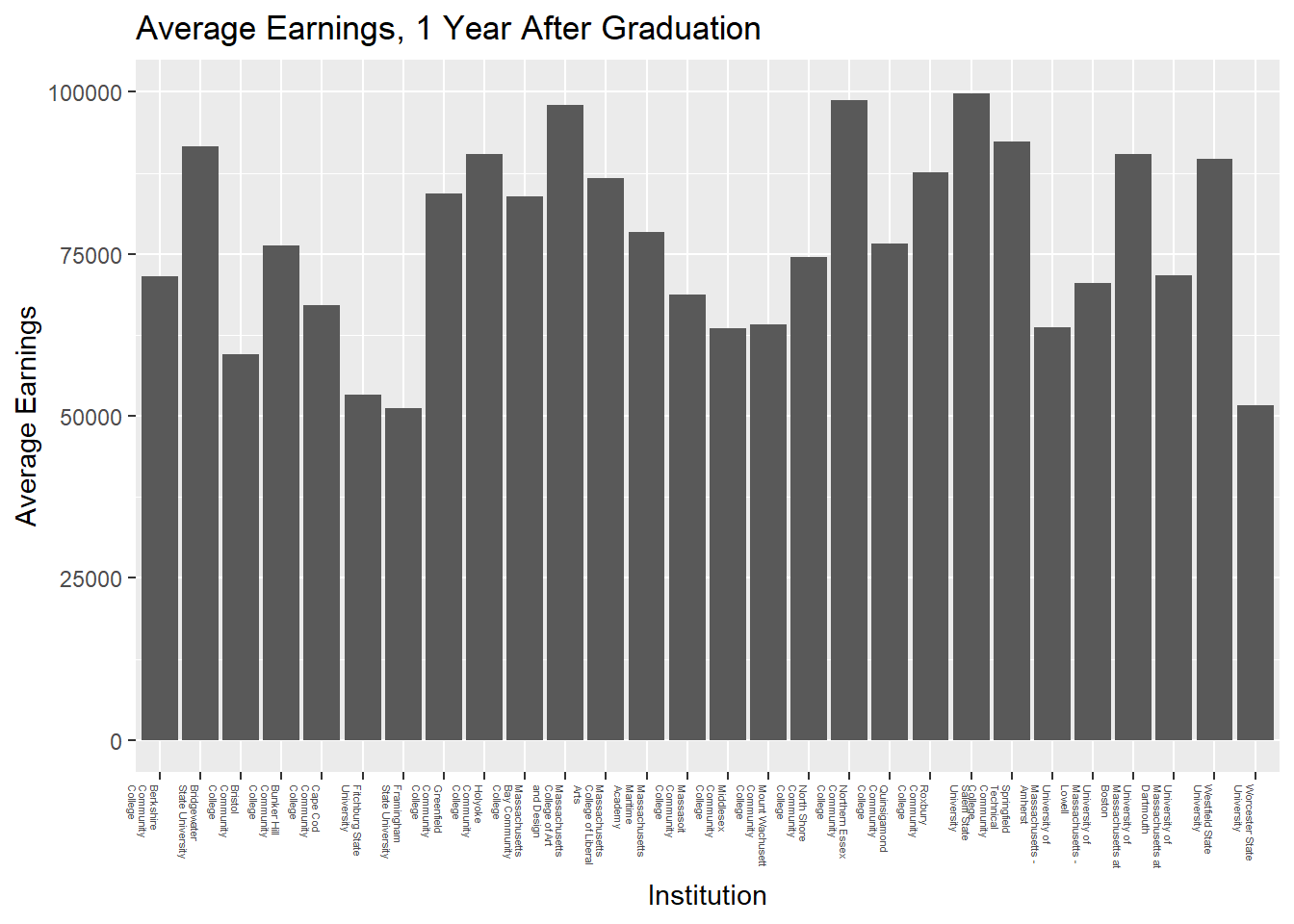
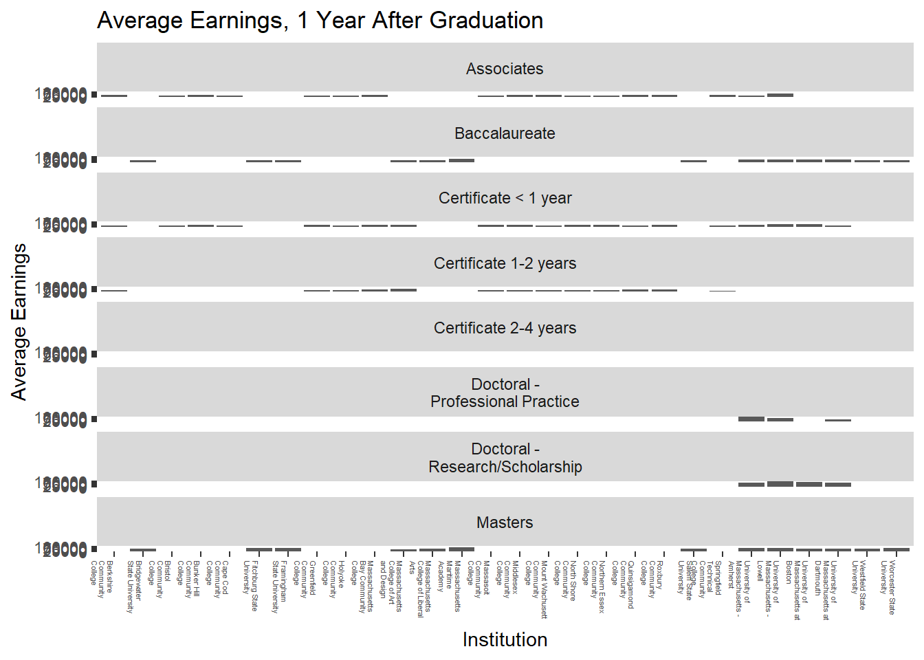
Question 1: It is clear in the data that there exists an increasing relationship between credentials and earnings. Further, as credentials increase toward the doctoral level, earnings increase. This is corroborated in Table 1 below. For example, Doctoral graduates earn more than twice (on average, around $80k, 1 year after graduation) than Baccalaureate graduates (on average, around $40k, 1 year after graduation). With the exception of Certificates 1-2 years, and both types of doctoral degrees, the data is skewed right. This implies that the earnings data has a peak on the left side of the graph with gradual decrease on the right.
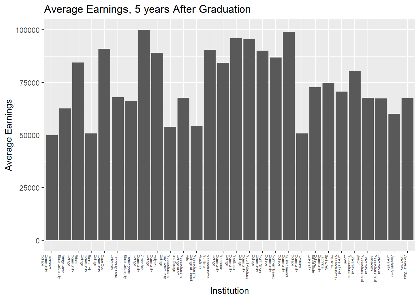
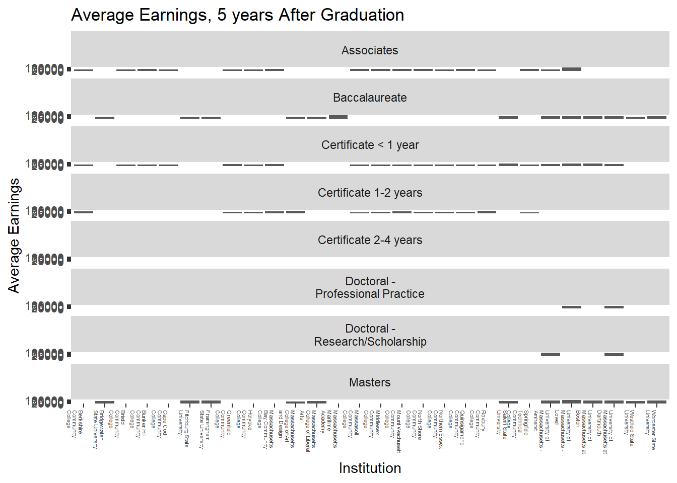
Question 2: It is also evident in the data that earnings increase with time elapsed since graduation. As seen in the data below:
Summary Statistics, Year 1, p50 Earnings Min. 1st Qu. Median Mean 3rd Qu. Max. NA’s 22214 34095 38097 46229 55442 120621 10
Summary Statistics, Year 5, p50 Earnings Min. 1st Qu. Median Mean 3rd Qu. Max. NA’s 31422 47280 53655 60603 70968 138314 10
Note the increase in mean earnings from $38,097 in Year 1 to $53,655 by Year 5.
Question 3: My conjecture is that STEM fields are most lucrative, at any credential level. With strong labor markets in STEM professions, the postsecondary employment outcomes are strongest for those in STEM fields. I will later perform a check using UMass Amherst BA earnings data by academic field.
Close Up: Earnings of BA Economics Graduates
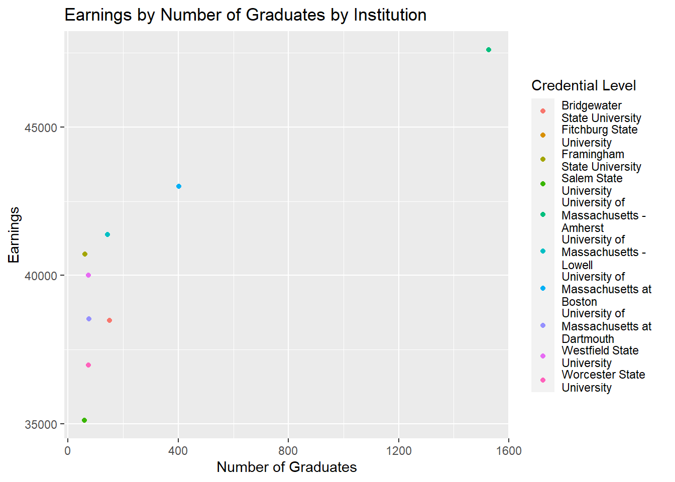
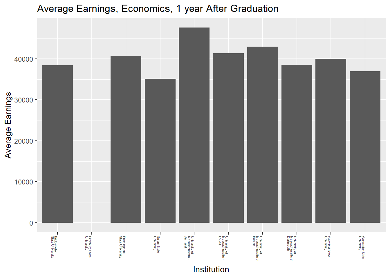
Out of curiousity, I proceeded to analyze the earnings patterns of BA Economics graduates in the MA public system. I found that of all the MA public Economics BA granting institutions, University of Massachusetts Amherst recorded the highest earnings at 47610 after 1 year of graduation. What is interesting to note is that earnings of Year 1 graduates of the UMass segment were consistently higher than state university This pattern did not extend to the 5 year mark, earnings of BA graduates were higher at the UMass campuses (with the exception of UMass Dartmouth) and highest at UMass Amherst , with Bridgewater State, Framingham State and Worcester State all showing earnings of over 60000.
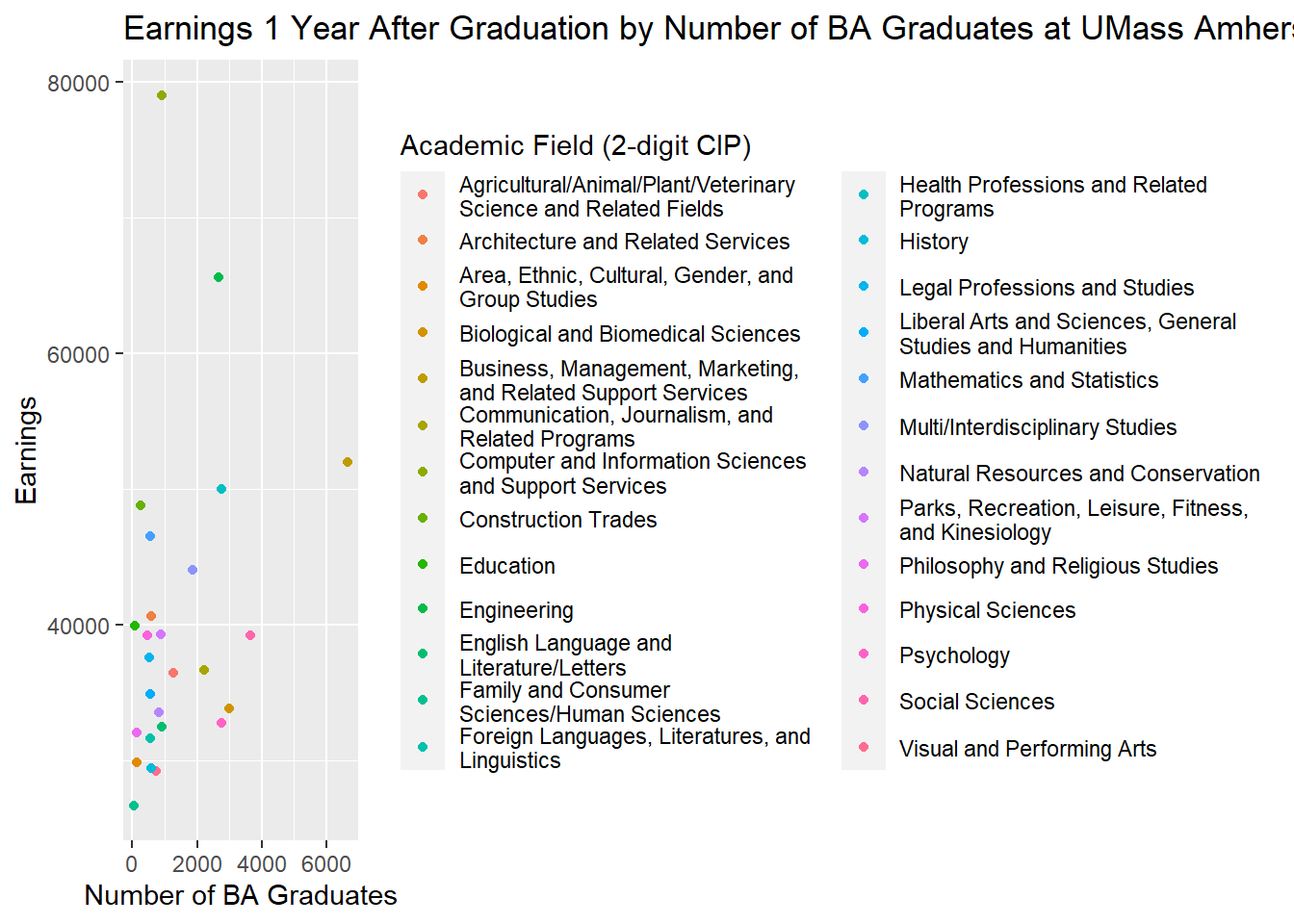
Close Up: Earnings of UMass Amherst BA Graduates
In general, graduates of UMass Amherst have the highest earnings of graduates of any public higher education institution in Massachusetts. Fields that are particularly lucrative are, in descending order, Computer Science, Engineering, Business and Health Professions. Conversely, fields such as Human Sciences, Visual and Performing Arts and History are the least lucrative fields. This is not a shock and corroborates common conventional thought and practices about what fields are most lucrative.
Data Wrangling
Code
# Find the number of rows and columns in the datasetnrow(pseo_ma_SANDBOX)
[1] 12639
Code
ncol(pseo_ma_SANDBOX)
[1] 48
Code
# Convert to numeric, 1 year after graduationpseo_ma_SANDBOX$y1_grads_earn =as.numeric((pseo_ma_SANDBOX$y1_grads_earn))pseo_ma_SANDBOX$y1_ipeds_count =as.numeric((pseo_ma_SANDBOX$y1_ipeds_count))pseo_ma_SANDBOX$y1_p50_earnings =as.numeric((pseo_ma_SANDBOX$y1_p50_earnings))
Code
# Convert to numeric, five years after graduationpseo_ma_SANDBOX$y5_grads_earn =as.numeric((pseo_ma_SANDBOX$y5_grads_earn))pseo_ma_SANDBOX$y5_ipeds_count =as.numeric((pseo_ma_SANDBOX$y5_ipeds_count))pseo_ma_SANDBOX$y5_p50_earnings =as.numeric((pseo_ma_SANDBOX$y5_p50_earnings))
## Descriptive Statistics

::: {.cell}

```{.r .cell-code}
# Filter data

pseo_filtered_two <-filter(pseo_ma_SANDBOX, pseo_ma_SANDBOX$label_cipcode=="All Instructional Programs" & pseo_ma_SANDBOX$label_grad_cohort== "All Cohorts")
View(pseo_filtered_two)
:::
Code
# Summary Statistics, 1 year after Graduationy1gradsearnSummary <-summary(pseo_filtered_two$y1_grads_earn, na.rm=T)print(y1gradsearnSummary)
   Min. 1st Qu.  Median    Mean 3rd Qu.    Max.    NA's
   34.0   186.5   708.0  2403.7  2315.0 35472.0      10
   Min. 1st Qu.  Median    Mean 3rd Qu.    Max.    NA's
  31422   47280   53655   60603   70968  138314      10
Code
``# 1 year Earnings by Credential- Mean and Medianpseo_filtered_two %>%group_by(pseo_filtered_two$label_degree_level) %>%summarise(Mean_Earnings=mean(y1_p50_earnings, na.rm=T), Median_Earnings=median(y1_p50_earnings, na.rm=T))
Error: attempt to use zero-length variable name
Code
# Filter data-- just BA degreespseo_filtered <-filter(pseo_ma_SANDBOX, pseo_ma_SANDBOX$label_degree_level=="Baccalaureate", pseo_ma_SANDBOX$label_cipcode!="All Instructional Programs"& pseo_ma_SANDBOX$label_grad_cohort=="All Cohorts")`
# Bar Chart, Mean Earnings One Year After Graduation all and by Credential Level options(scipen =999)vis_y1_p50_earnings <-ggplot(pseo_filtered_two, aes(x=label_institution, y=y1_p50_earnings)) +geom_bar(stat="identity") +stat_summary(fun = mean, geom ="col") +ggtitle("Average Earnings, 1 Year After Graduation") +xlab("Institution") +ylab("Average Earnings") +theme(axis.text.x=element_text(size=4, angle =-90, hjust =0)) +scale_y_continuous(limits=c(0,100000))print(vis_y1_p50_earnings)
# Bar Chart, Mean Earnings 5 Years After Graduation (all) and by Credential Leveloptions(scipen =999)vis_y5_p50_earnings <-ggplot(pseo_filtered_two, aes(x=label_institution, y=y5_p50_earnings)) +geom_bar(stat="identity") +stat_summary(fun = mean, geom ="col") +ggtitle("Average Earnings, 5 years After Graduation") +xlab("Institution") +ylab("Average Earnings") +theme(axis.text.x=element_text(size=4, angle =-90, hjust =0)) +scale_y_continuous(limits=c(0,100000))print(vis_y5_p50_earnings)
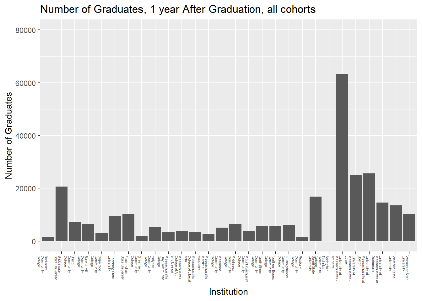
# Bar Graph of Number of Graduatesoptions(scipen =999)pseo_filtered_two$y1_ipeds_count <-as.numeric(pseo_filtered_two$y1_ipeds_count)vis_y1_graduates <-ggplot(pseo_filtered_two, aes(x=label_institution, y=y1_ipeds_count)) +geom_bar(stat="identity") +stat_summary(fun = mean, geom ="col") +ggtitle("Number of Graduates, 1 year After Graduation, all cohorts") +xlab("Institution") +ylab("Number of Graduates") +theme(axis.text.x=element_text(size=4, angle =-90, hjust =0)) +scale_y_continuous(limits =c(0, 80000))print(vis_y1_graduates)
# Filter for Baccalaureate Economics degreeslibrary(dplyr)pseo_filtered_econ<-filter(pseo_ma_SANDBOX, pseo_ma_SANDBOX$label_degree_level=="Baccalaureate"& pseo_ma_SANDBOX$label_cipcode=="Economics"& pseo_ma_SANDBOX$label_grad_cohort=="All Cohorts")# Scatterplot of Bachelors in Economics, all institutionsvis_600 <-ggplot(pseo_filtered_econ, aes(x=y1_grads_earn, y=y1_p50_earnings, color=label_institution)) +geom_point() +labs(y="Earnings", x="Number of Graduates", color="Credential Level", title ="Earnings by Number of Graduates by Institution")print(vis_600)
# Bar of Bachelors in Economicspseo_filtered_econ %>%group_by(pseo_filtered_econ$label_degree_level, pseo_filtered_econ$label_institution) %>%summarise(Mean=mean(y1_p50_earnings, na.rm=T), Median=median(y1_p50_earnings, na.rm=T))
# 1 year earnings for BAs by 2-digit CIP Code at UMass Amherst- Scatterplotlibrary(dplyr)pseo_filtered_three <-filter(pseo_ma_SANDBOX, pseo_ma_SANDBOX$institution=="00222100"& pseo_ma_SANDBOX$label_degree_level=="Baccalaureate"& pseo_ma_SANDBOX$cip_level=="2"& pseo_ma_SANDBOX$label_grad_cohort=="All Cohorts")vis_650 <-ggplot(pseo_filtered_three, aes(x=y1_grads_earn, y=y1_p50_earnings, color=label_cipcode)) +geom_point() +labs(y="Earnings", x="Number of BA Graduates", color="Academic Field (2-digit CIP)", title ="Earnings 1 Year After Graduation by Number of BA Graduates at UMass Amherst by Academic Field")print(vis_650)
# A tibble: 26 x 49
# Groups:   pseo_filtered_three$label_cipcode [26]
   agg_level_pseo label_agg_level_pseo   inst_level label_inst_level institution
            <dbl> <chr>                  <chr>      <chr>            <chr>
 1             40 "Degree Level * CIP\r~ I          Institution      00222100
 2             40 "Degree Level * CIP\r~ I          Institution      00222100
 3             40 "Degree Level * CIP\r~ I          Institution      00222100
 4             40 "Degree Level * CIP\r~ I          Institution      00222100
 5             40 "Degree Level * CIP\r~ I          Institution      00222100
 6             40 "Degree Level * CIP\r~ I          Institution      00222100
 7             40 "Degree Level * CIP\r~ I          Institution      00222100
 8             40 "Degree Level * CIP\r~ I          Institution      00222100
 9             40 "Degree Level * CIP\r~ I          Institution      00222100
10             40 "Degree Level * CIP\r~ I          Institution      00222100
# i 16 more rows
# i 44 more variables: label_institution <chr>,
#   `Degree\r\nAward\r\nLevel` <chr>, label_degree_level <chr>,
#   cip_level <chr>, label_cip_level <chr>, cipcode <chr>, label_cipcode <chr>,
#   grad_cohort <chr>, label_grad_cohort <chr>, grad_cohort_years <chr>,
#   label_grad_cohort_years <chr>, geo_level <chr>, label_geo_level <chr>,
#   geography <chr>, label_geography <chr>, ind_level <chr>, ...
Code
summarise(Mean=mean(y1_p50_earnings, na.rm=T))
Error in mean(y1_p50_earnings, na.rm = T): object 'y1_p50_earnings' not found
Critical Reflection
What I learned from this project confirmed conventional knowledge and axioms. For example, my analyses confirmed that earnings generally increase with credential level, earnings generally increase with time since graduation elapsed, and earnings in STEM fields are generally higher than other fields. The limitations of my analysis is that I did not break down my analysis demographically. I expect that the Census Bureau will provide this disaggregated data in time. Given the recent Supreme Court decision on affirmative action, I would conjecture that such employment outcomes data disaggregated by race/ethnicity would be a useful and timely addition to the dataset and further analysis. Further statistical analysis could test the relationship between credential level and earnings, and test if they are correlated as well. Further, we could check for a statistical relationship between earnings and race/ethnicity. In addition, unit record data would be very interesting for analysis using panel data methods.
References
Census Bureau (2023). Post-secondary Employment Outcomes: Massachusetts. [Dataset]. https://lehd.ces.census.gov/data/pseo_experimental.html
Wickham, H., & Grolemund, G. (2016). R for data science: Visualize, model, transform, tidy, and import data. OReilly Media.
Source Code
---title: "Final Project"author: "Moira Chiong"description: "Final Project: Census PSEO Analysis"date: "7/13/2023"format: html: toc: true code-fold: true code-copy: true code-tools: true---```{r setup, include=FALSE} knitr::opts_chunk$set(warning =FALSE, message =FALSE) ## Read in Data```{r}setwd("C:/Users/chion/OneDrive/Desktop/DACSS 601/DACSS_601_Summer2023_Sec1/posts")library(readxl)library(tidyverse)library(dplyr)library(ggplot2)pseo_ma_SANDBOX <- read_excel("datafolderMoiraChiong/pseo_ma_SANDBOX.xlsx")pseo_ma_SANDBOX```## IntroductionFor my final project, I used the Census Bureau Post-Secondary Employment Outcomes (PSEO) database filtered for Massachusetts. This database cites the employment outcomes (earnings 1, 5 and 10 years after graduation) for all public Massachusetts higher education institutions. The data set provides postsecondary employment outcomes for graduates at all credential levels, from certificate to doctorate. The data is divided into three to five year cohorts, ranging from 2001-2018. In addition, there are tabulations of number of graduates and number of employed graduates in the data set.Some limitations of this data set are that it is not disaggregated by demographic variables such as race/ethnicity, gender, age or Pell status. This makes a truly nuanced study of the variables and research questions less possible with the present data set. It is my hope that new iterations of this data set will include such demographic variables. ## Potential Research QuestionsThe following questions are intended to uncover patterns in the PSEO data. While robust analysis of patterns in the data may require advanced statistical analysis, the data analysis completed in the project do reveal underlying general patterns.My research questions are as follows:1. What is the relationship between credential level and earnings? 2. What is the relationship between time elapsed since graduation and earnings? Do earnings grow as more years after graduation elapse?3. What is the relationship between academic field of study and earnings?Questions for further research: What is the relationship between race/ethnicity, age, Pell status and earnings?## Notes on Code- Data Analysis and Answers to Questions 1-3Question 1: It is clear in the data that there exists an increasing relationship between credentials and earnings. Further, as credentials increase toward the doctoral level, earnings increase. This is corroborated in Table 1 below. For example, Doctoral graduates earn more than twice (on average, around $80k, 1 year after graduation) than Baccalaureate graduates (on average, around $40k, 1 year after graduation). With the exception of Certificates 1-2 years, and both types of doctoral degrees, the data is skewed right. This implies that the earnings data has a peak on the left side of the graph with gradual decrease on the right.Question 2: It is also evident in the data that earnings increase with time elapsed since graduation. As seen in the data below:Summary Statistics, Year 1, p50 Earnings Min. 1st Qu. Median Mean 3rd Qu. Max. NA's 22214 34095 38097 46229 55442 120621 10 Summary Statistics, Year 5, p50 EarningsMin. 1st Qu. Median Mean 3rd Qu. Max. NA's 314224728053655606037096813831410Note the increase in mean earnings from $38,097in Year 1 to $53,655 by Year 5.Question 3: My conjecture is that STEM fields are most lucrative, at any credential level. With strong labor markets in STEM professions, the postsecondary employment outcomes are strongest for those in STEM fields. I will later perform a check using UMass Amherst BA earnings data by academic field. # Close Up: Earnings of BA Economics GraduatesOut of curiousity, I proceeded to analyze the earnings patterns of BA Economics graduates in the MA public system. I found that of all the MA public Economics BA granting institutions, University of Massachusetts Amherst recorded the highest earnings at 47610 after 1 year of graduation. What is interesting to note is that earnings of Year 1 graduates of the UMass segment were consistently higher than state university This pattern did not extend to the 5 year mark, earnings of BA graduates were higher at the UMass campuses (with the exception of UMass Dartmouth) and highest at UMass Amherst , with Bridgewater State, Framingham State and Worcester State all showing earnings of over 60000.# Close Up: Earnings of UMass Amherst BA GraduatesIn general, graduates of UMass Amherst have the highest earnings of graduates of any public higher education institution in Massachusetts. Fields that are particularly lucrative are, in descending order, Computer Science, Engineering, Business and Health Professions. Conversely, fields such as Human Sciences, Visual and Performing Arts and History are the least lucrative fields. This is not a shock and corroborates common conventional thought and practices about what fields are most lucrative. ## Data Wrangling```{r}# Find the number of rows and columns in the datasetnrow(pseo_ma_SANDBOX)ncol(pseo_ma_SANDBOX)``````{r}# Convert to numeric, 1 year after graduationpseo_ma_SANDBOX$y1_grads_earn = as.numeric((pseo_ma_SANDBOX$y1_grads_earn))pseo_ma_SANDBOX$y1_ipeds_count = as.numeric((pseo_ma_SANDBOX$y1_ipeds_count))pseo_ma_SANDBOX$y1_p50_earnings = as.numeric((pseo_ma_SANDBOX$y1_p50_earnings))``````{r}# Convert to numeric, five years after graduationpseo_ma_SANDBOX$y5_grads_earn = as.numeric((pseo_ma_SANDBOX$y5_grads_earn))pseo_ma_SANDBOX$y5_ipeds_count = as.numeric((pseo_ma_SANDBOX$y5_ipeds_count))pseo_ma_SANDBOX$y5_p50_earnings = as.numeric((pseo_ma_SANDBOX$y5_p50_earnings))``````## Descriptive Statistics```{r}# Filter datapseo_filtered_two <-filter(pseo_ma_SANDBOX, pseo_ma_SANDBOX$label_cipcode=="All Instructional Programs"& pseo_ma_SANDBOX$label_grad_cohort=="All Cohorts")View(pseo_filtered_two)``````{r}# Summary Statistics, 1 year after Graduationy1gradsearnSummary <-summary(pseo_filtered_two$y1_grads_earn, na.rm=T)print(y1gradsearnSummary)y1ipedscountSummary <-summary(pseo_filtered_two$y1_ipeds_count, na.rm=T)print(y1ipedscountSummary)y1p50earningsSummary <-summary(pseo_filtered_two$y1_p50_earnings, na.rm=T)print(y1p50earningsSummary)# Find summary statistics, 5 years after graduationy5gradsearnSummary <-summary(pseo_filtered_two$y5_grads_earn, na.rm=T)print(y5gradsearnSummary)y5ipedscountSummary <-summary(pseo_filtered_two$y5_ipeds_count, na.rm=T)print(y5ipedscountSummary)y5p50earningsSummary <-summary(pseo_filtered_two$y5_p50_earnings, na.rm=T)print(y5p50earningsSummary)``````{r}``# 1 year Earnings by Credential- Mean and Medianpseo_filtered_two %>%group_by(pseo_filtered_two$label_degree_level) %>%summarise(Mean_Earnings=mean(y1_p50_earnings, na.rm=T), Median_Earnings=median(y1_p50_earnings, na.rm=T))``````{r}# Filter data-- just BA degreespseo_filtered <-filter(pseo_ma_SANDBOX, pseo_ma_SANDBOX$label_degree_level=="Baccalaureate", pseo_ma_SANDBOX$label_cipcode!="All Instructional Programs"& pseo_ma_SANDBOX$label_grad_cohort=="All Cohorts")````## Data Visualization Code```{r}# Bar Chart, Mean Earnings One Year After Graduation all and by Credential Level options(scipen = 999)vis_y1_p50_earnings <- ggplot(pseo_filtered_two, aes(x=label_institution, y=y1_p50_earnings)) + geom_bar(stat="identity") + stat_summary(fun = mean, geom = "col") + ggtitle("Average Earnings, 1 Year After Graduation") + xlab("Institution") + ylab("Average Earnings") + theme(axis.text.x=element_text(size=4, angle = -90, hjust = 0)) + scale_y_continuous(limits=c(0,100000)) print(vis_y1_p50_earnings) vis_y1_p50_earnings + facet_wrap( ~ label_degree_level, ncol=1)# Bar Chart, Mean Earnings 5 Years After Graduation (all) and by Credential Leveloptions(scipen = 999)vis_y5_p50_earnings <- ggplot(pseo_filtered_two, aes(x=label_institution, y=y5_p50_earnings)) + geom_bar(stat="identity") + stat_summary(fun = mean, geom = "col") + ggtitle("Average Earnings, 5 years After Graduation") + xlab("Institution") + ylab("Average Earnings") + theme(axis.text.x=element_text(size=4, angle = -90, hjust = 0)) + scale_y_continuous(limits=c(0,100000)) print(vis_y5_p50_earnings) vis_y5_p50_earnings + facet_wrap( ~ label_degree_level, ncol=1)``````{r}# Bar Graph of Number of Graduatesoptions(scipen = 999)pseo_filtered_two$y1_ipeds_count <- as.numeric(pseo_filtered_two$y1_ipeds_count)vis_y1_graduates <- ggplot(pseo_filtered_two, aes(x=label_institution, y=y1_ipeds_count)) + geom_bar(stat="identity") + stat_summary(fun = mean, geom = "col") + ggtitle("Number of Graduates, 1 year After Graduation, all cohorts") + xlab("Institution") + ylab("Number of Graduates") + theme(axis.text.x=element_text(size=4, angle = -90, hjust = 0)) +scale_y_continuous(limits = c(0, 80000)) print(vis_y1_graduates) vis_y1_graduates + facet_wrap( ~ label_degree_level, ncol=1)# Filter for Baccalaureate Economics degreeslibrary(dplyr)pseo_filtered_econ<-filter(pseo_ma_SANDBOX, pseo_ma_SANDBOX$label_degree_level=="Baccalaureate" & pseo_ma_SANDBOX$label_cipcode=="Economics" & pseo_ma_SANDBOX$label_grad_cohort== "All Cohorts")# Scatterplot of Bachelors in Economics, all institutionsvis_600 <-ggplot(pseo_filtered_econ, aes(x=y1_grads_earn, y=y1_p50_earnings, color=label_institution)) +geom_point() +labs(y= "Earnings", x= "Number of Graduates", color= "Credential Level", title = "Earnings by Number of Graduates by Institution")print(vis_600)pseo_filtered_econ %>%group_by(pseo_filtered_econ$label_degree_level, pseo_filtered_econ$label_institution) %>%summarise(Mean=mean(y1_p50_earnings, na.rm=T), Median=median(y1_p50_earnings, na.rm=T))pseo_filtered_econ %>%group_by(pseo_filtered_econ$label_institution) %>%summarise(Mean=mean(y5_p50_earnings, na.rm=T), Median=median(y5_p50_earnings, na.rm=T))``````{r}# Bar of Bachelors in Economicspseo_filtered_econ %>%group_by(pseo_filtered_econ$label_degree_level, pseo_filtered_econ$label_institution) %>%summarise(Mean=mean(y1_p50_earnings, na.rm=T), Median=median(y1_p50_earnings, na.rm=T))`````````{r}options(scipen =999)vis_y1_econ <-ggplot(pseo_filtered_econ, aes(x=label_institution, y=y1_p50_earnings)) +geom_bar(stat="identity") +ggtitle("Average Earnings, Economics, 1 year After Graduation") +xlab("Institution") +ylab("Average Earnings") +theme(axis.text.x=element_text(size=4, angle =-90, hjust =0)) print(vis_y1_econ)``````{r}# 1 year earnings for BAs by 2-digit CIP Code at UMass Amherst- Scatterplotlibrary(dplyr)pseo_filtered_three <-filter(pseo_ma_SANDBOX, pseo_ma_SANDBOX$institution=="00222100"& pseo_ma_SANDBOX$label_degree_level=="Baccalaureate"& pseo_ma_SANDBOX$cip_level=="2"& pseo_ma_SANDBOX$label_grad_cohort=="All Cohorts")vis_650 <-ggplot(pseo_filtered_three, aes(x=y1_grads_earn, y=y1_p50_earnings, color=label_cipcode)) +geom_point() +labs(y="Earnings", x="Number of BA Graduates", color="Academic Field (2-digit CIP)", title ="Earnings 1 Year After Graduation by Number of BA Graduates at UMass Amherst by Academic Field")print(vis_650)``````{r}library(dplyr)pseo_filtered_three <-filter(pseo_ma_SANDBOX, pseo_ma_SANDBOX$institution=="00222100"& pseo_ma_SANDBOX$label_degree_level=="Baccalaureate"& pseo_ma_SANDBOX$cip_level=="2"& pseo_ma_SANDBOX$label_grad_cohort=="All Cohorts")# Bachelor's Earnings by CIP Code, UMass Amherstpseo_filtered_three %>%group_by(pseo_filtered_three$label_cipcode)summarise(Mean=mean(y1_p50_earnings, na.rm=T))```## Critical ReflectionWhat I learned from this project confirmed conventional knowledge and axioms. For example, my analyses confirmed that earnings generally increase with credential level, earnings generally increase with time since graduation elapsed, and earnings in STEM fields are generally higher than other fields. The limitations of my analysis is that I did not break down my analysis demographically. I expect that the Census Bureau will provide this disaggregated data in time. Given the recent Supreme Court decision on affirmative action, I would conjecture that such employment outcomes data disaggregated by race/ethnicity would be a useful and timely addition to the dataset and further analysis. Further statistical analysis could test the relationship between credential level and earnings, and test if they are correlated as well. Further, we could check for a statistical relationship between earnings and race/ethnicity. In addition, unit record data would be very interesting for analysis using panel data methods. ## ReferencesCensus Bureau (2023). Post-secondary Employment Outcomes: Massachusetts. [Dataset]. https://lehd.ces.census.gov/data/pseo_experimental.htmlWickham, H., & Grolemund, G. (2016). R for data science: Visualize, model, transform, tidy, and import data. OReilly Media.