Code
library(ggplot2)
library(dplyr)
library(tidyr)
library(tidyverse)
library(caret)
library(randomForest)
library(lubridate)
data <- read_csv("_data/hotel_bookings.csv")
knitr::opts_chunk$set(echo = TRUE)library(ggplot2)
library(dplyr)
library(tidyr)
library(tidyverse)
library(caret)
library(randomForest)
library(lubridate)
data <- read_csv("_data/hotel_bookings.csv")
knitr::opts_chunk$set(echo = TRUE)This project focuses on the comprehensive analysis of a hotel booking dataset, consisting of detailed information about bookings made at a city hotel and a resort hotel. By employing various data exploration and visualization techniques, we aim to uncover patterns and gain insights into hotel booking behaviors. The dataset spans the years 2015 to 2017 and has undergone preprocessing steps to ensure data quality. This project not only aims to answer research queries but also aims to provide a clear and understandable narrative for individuals without prior expertise in the field.
Introduction
The hotel industry is an essential component of the tourism sector, and understanding booking behaviors is crucial for optimizing hotel operations and enhancing customer satisfaction. This project utilizes a comprehensive hotel booking dataset to analyze and extract valuable insights regarding booking trends, customer preferences, and other relevant factors.
Data Exploration and Understanding
Initially, we explored the hotel booking dataset, gaining an understanding of its structure and variables. Each variable was carefully examined to determine its significance in the analysis. Irrelevant columns were removed, and missing values were handled appropriately. Additionally, date fields were converted to the correct data type to facilitate further analysis.
Research Questions
Based on the dataset exploration, several key research questions were formulated to guide our analysis. These questions revolve around various aspects of hotel bookings, such as booking patterns, customer demographics, and factors influencing booking cancellations.
datasummary(data) hotel is_canceled lead_time arrival_date_year
Length:119390 Min. :0.0000 Min. : 0 Min. :2015
Class :character 1st Qu.:0.0000 1st Qu.: 18 1st Qu.:2016
Mode :character Median :0.0000 Median : 69 Median :2016
Mean :0.3704 Mean :104 Mean :2016
3rd Qu.:1.0000 3rd Qu.:160 3rd Qu.:2017
Max. :1.0000 Max. :737 Max. :2017
arrival_date_month arrival_date_week_number arrival_date_day_of_month
Length:119390 Min. : 1.00 Min. : 1.0
Class :character 1st Qu.:16.00 1st Qu.: 8.0
Mode :character Median :28.00 Median :16.0
Mean :27.17 Mean :15.8
3rd Qu.:38.00 3rd Qu.:23.0
Max. :53.00 Max. :31.0
stays_in_weekend_nights stays_in_week_nights adults
Min. : 0.0000 Min. : 0.0 Min. : 0.000
1st Qu.: 0.0000 1st Qu.: 1.0 1st Qu.: 2.000
Median : 1.0000 Median : 2.0 Median : 2.000
Mean : 0.9276 Mean : 2.5 Mean : 1.856
3rd Qu.: 2.0000 3rd Qu.: 3.0 3rd Qu.: 2.000
Max. :19.0000 Max. :50.0 Max. :55.000
children babies meal country
Min. : 0.0000 Min. : 0.000000 Length:119390 Length:119390
1st Qu.: 0.0000 1st Qu.: 0.000000 Class :character Class :character
Median : 0.0000 Median : 0.000000 Mode :character Mode :character
Mean : 0.1039 Mean : 0.007949
3rd Qu.: 0.0000 3rd Qu.: 0.000000
Max. :10.0000 Max. :10.000000
NA's :4
market_segment distribution_channel is_repeated_guest
Length:119390 Length:119390 Min. :0.00000
Class :character Class :character 1st Qu.:0.00000
Mode :character Mode :character Median :0.00000
Mean :0.03191
3rd Qu.:0.00000
Max. :1.00000
previous_cancellations previous_bookings_not_canceled reserved_room_type
Min. : 0.00000 Min. : 0.0000 Length:119390
1st Qu.: 0.00000 1st Qu.: 0.0000 Class :character
Median : 0.00000 Median : 0.0000 Mode :character
Mean : 0.08712 Mean : 0.1371
3rd Qu.: 0.00000 3rd Qu.: 0.0000
Max. :26.00000 Max. :72.0000
assigned_room_type booking_changes deposit_type agent
Length:119390 Min. : 0.0000 Length:119390 Length:119390
Class :character 1st Qu.: 0.0000 Class :character Class :character
Mode :character Median : 0.0000 Mode :character Mode :character
Mean : 0.2211
3rd Qu.: 0.0000
Max. :21.0000
company days_in_waiting_list customer_type adr
Length:119390 Min. : 0.000 Length:119390 Min. : -6.38
Class :character 1st Qu.: 0.000 Class :character 1st Qu.: 69.29
Mode :character Median : 0.000 Mode :character Median : 94.58
Mean : 2.321 Mean : 101.83
3rd Qu.: 0.000 3rd Qu.: 126.00
Max. :391.000 Max. :5400.00
required_car_parking_spaces total_of_special_requests reservation_status
Min. :0.00000 Min. :0.0000 Length:119390
1st Qu.:0.00000 1st Qu.:0.0000 Class :character
Median :0.00000 Median :0.0000 Mode :character
Mean :0.06252 Mean :0.5714
3rd Qu.:0.00000 3rd Qu.:1.0000
Max. :8.00000 Max. :5.0000
reservation_status_date
Min. :2014-10-17
1st Qu.:2016-02-01
Median :2016-08-07
Mean :2016-07-30
3rd Qu.:2017-02-08
Max. :2017-09-14
The dataset contains information about hotel bookings, including various features such as cancellation status, lead time, arrival date, duration of stay, number of adults, children, and babies, meal type, country of origin, market segment, distribution channel, previous cancellations and bookings, reserved room type, assigned room type, booking changes, deposit type, agent, company, days in waiting list, customer type, average daily rate (ADR), required car parking spaces, total number of special requests, reservation status, and reservation status date.
The dataset consists of 119,390 records and provides a comprehensive overview of hotel bookings. It spans a period from 2015 to 2017, capturing data on various aspects of guest preferences and booking patterns. The dataset allows for exploration and analysis of factors that may influence cancellations, room type preferences, special requests, pricing strategies, and other aspects related to hotel bookings.
However, it is important to note that the dataset has some limitations. It does not include information about specific demographic characteristics of guests, such as age, gender, or income level. Additionally, the dataset does not provide detailed information about the reasons for cancellations or the specific amenities and services requested as part of special requests. Exploring these factors would provide a more comprehensive understanding of guest behavior and preferences.
Overall, the dataset provides a valuable foundation for analyzing hotel booking trends and understanding customer behavior, but additional data and analysis may be necessary to address more specific research questions and delve deeper into the factors influencing hotel pricing strategies and guest preferences.
in this part we done three things
Now, we can see the new data set.
# 1. Remove irrelevant or redundant columns
data <- data %>%
select(-c(agent, company))
# 2. Handle missing values: replace the missing values of the list of values with the average value
data$children[is.na(data$children)] <- mean(data$children, na.rm = TRUE)
# Note: we assume the day of each observation to be the 1st
data <- data %>% mutate(arrival_date = ymd(paste(arrival_date_year, arrival_date_month, arrival_date_day_of_month, sep = "-")))
#drop the original Year and Month columns
data <- data %>% select(-arrival_date_year, -arrival_date_month, -arrival_date_day_of_month)
dataThe dataset that we are analyzing is about hotel bookings. It contains 119,390 records, each representing a separate hotel booking. These bookings span from the year 2015 to 2017, covering various hotels, customers from different countries, and diverse market segments. It is a rich dataset providing various insights into hotel booking patterns, customer preferences, and booking cancellations.
This dataset comprises various information about hotel bookings. For each booking, the following attributes are provided:
hotel: Hotel (Resort Hotel or City Hotel) where the booking was made.is_canceled: Value indicating if the booking was canceled (1) or not (0).lead_time: Number of days that elapsed between the entering date of the booking into the Property Management System and the arrival date.arrival_date_year: Year of arrival date.arrival_date_month: Month of arrival date.arrival_date_week_number: Week number of year for arrival date.arrival_date_day_of_month: Day of arrival date.stays_in_weekend_nights: Number of weekend nights (Saturday or Sunday) the guest stayed or booked to stay at the hotel.stays_in_week_nights: Number of week nights (Monday to Friday) the guest stayed or booked to stay at the hotel.adults: Number of adults.children: Number of children.babies: Number of babies.meal: Type of meal booked.country: Country of origin of the booking.market_segment: Market segment designation.distribution_channel: Booking distribution channel.is_repeated_guest: Value indicating if the booking name was from a repeated guest (1) or not (0).previous_cancellations: Number of previous bookings that were cancelled by the customer prior to the current booking.previous_bookings_not_canceled: Number of previous bookings not cancelled by the customer prior to the current booking.reserved_room_type: Code of room type reserved.assigned_room_type: Code for the type of room assigned to the booking.booking_changes: Number of changes/amendments made to the booking from the moment the booking was entered on - the Property Management System until the moment of check-in or cancellation.deposit_type: Indication on if the customer made a deposit to guarantee the booking.agent: ID of the travel agency that made the booking.company: ID of the company/entity that made the booking or responsible for paying the booking.days_in_waiting_list: Number of days the booking was in the waiting list before it was confirmed to the customer.customer_type: Type of booking.adr: Average Daily Rate as defined by dividing the sum of all lodging transactions by the total number of staying nights.total_of_special_requests: Number of special requests made by the customer.reservation_status: Last reservation status, assuming one of three categories: Canceled, Check-Out, No-Show.reservation_status_date: Date at which the last status was set. The data are with very long content.# Plotting the number of bookings per month per year
data %>%
count(arrival_date_year = year(arrival_date), arrival_date_month = month(arrival_date, label = FALSE)) %>%
ggplot(aes(x = arrival_date_month, y = n, fill = as.factor(arrival_date_month))) +
geom_col() +
scale_x_continuous(breaks = 1:12, labels = month.abb) +
facet_wrap(~arrival_date_year) +
labs(x = "Month", y = "Number of Bookings", title = "Number of Bookings per Month per Year") +
theme_minimal()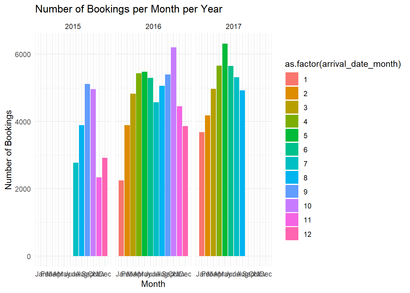
# Plotting the average lead time per month per year
data %>%
group_by(arrival_date_year = year(arrival_date), arrival_date_month = month(arrival_date, label = FALSE)) %>%
summarise(avg_lead_time = mean(lead_time, na.rm = TRUE), .groups = 'drop') %>%
ggplot(aes(x = arrival_date_month, y = avg_lead_time, fill = as.factor(arrival_date_month))) +
geom_col() +
scale_x_continuous(breaks = 1:12, labels = month.abb) +
facet_wrap(~arrival_date_year) +
labs(x = "Month", y = "Average Lead Time", title = "Average Lead Time per Month per Year") +
theme_minimal()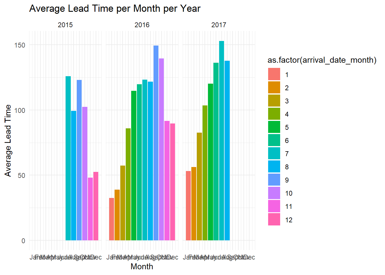
From the data provided, the busiest months for hotels, in terms of the number of bookings, tend to be May, June, and October in 2016 and April, May, and June in 2017. Notably, the month with the highest number of bookings was May in 2017 with 6300 bookings.
Regarding the relationship between lead time and busy periods, there seems to be a general trend that busier months have longer lead times. For instance, in 2016, October had the highest number of bookings and one of the longest average lead times (145 days). Similarly, in 2017, May had both the highest number of bookings and one of the longest lead times (119 days).
However, this is not always the case. In 2016, May had the longest lead time (150 days) but did not have the highest number of bookings (5250 bookings). In 2017, July had the longest lead time (151 days), but it was not the busiest month in terms of bookings.
Overall, while there appears to be some relationship between lead time and the number of bookings, the relationship is not consistent across all months. It’s possible that other factors also play a significant role in influencing booking patterns, such as seasonal events, holidays, and hotel pricing strategies, among others.
# Create a bar chart to visualize the popularity of different room types
data %>%
group_by(reserved_room_type) %>%
summarise(count = n()) %>%
ggplot(aes(x = reorder(reserved_room_type, -count), y = count)) +
geom_col(fill = "skyblue") +
labs(x = "Room Type", y = "Number of Bookings",
title = "Popularity of Room Types") +
theme_minimal()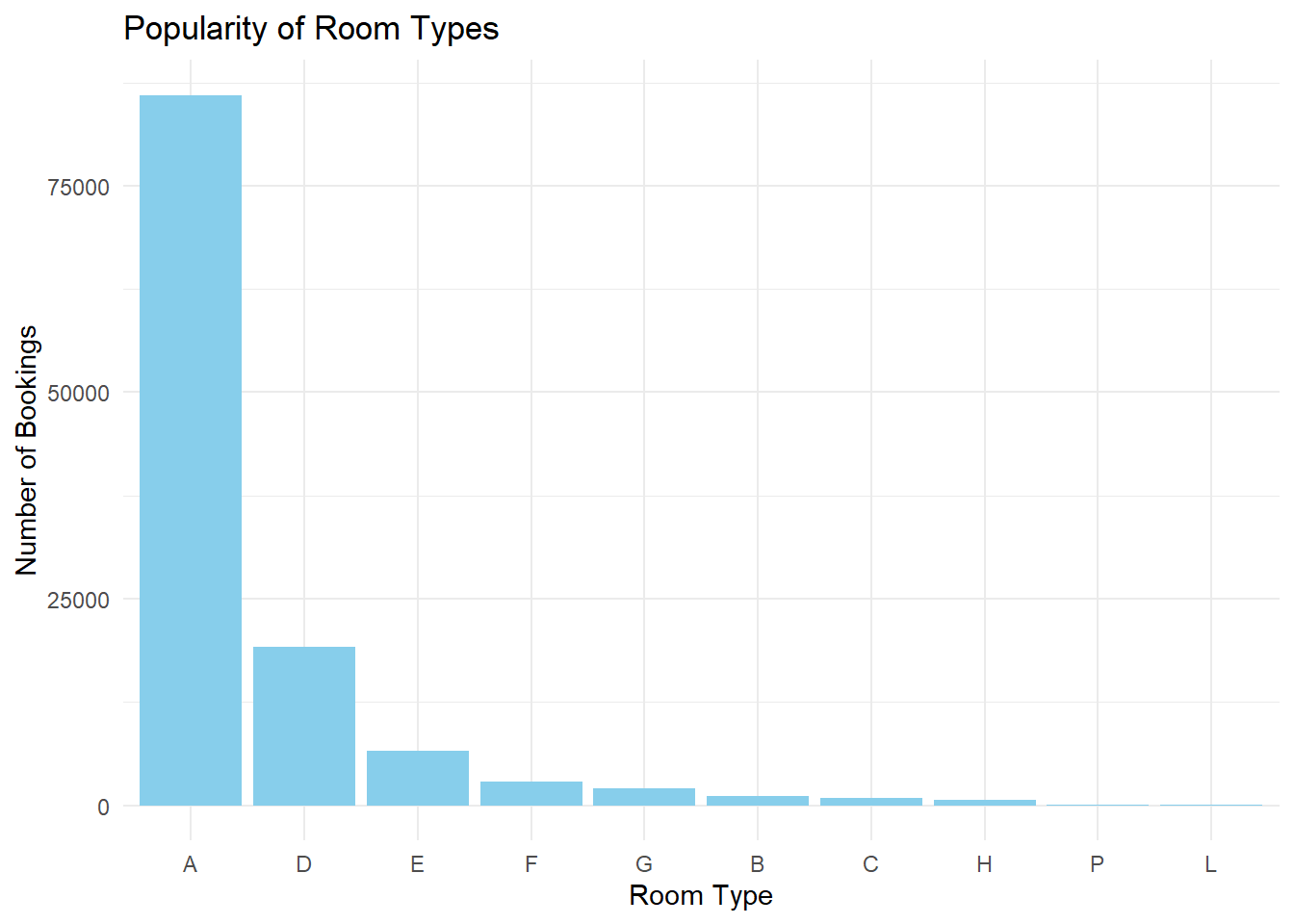
# Create a box plot to visualize the relationship between room type and number of adults
data %>%
ggplot(aes(x = reserved_room_type, y = adults)) +
geom_boxplot() +
labs(x = "Room Type", y = "Number of Adults",
title = "Room Type vs Number of Adults") +
theme_minimal()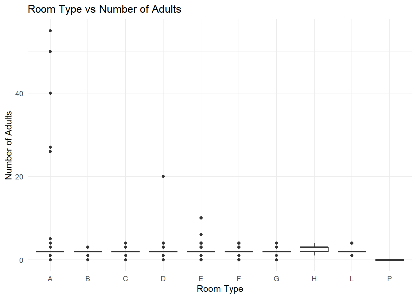
# Create a box plot to visualize the relationship between room type and number of children
data %>%
ggplot(aes(x = reserved_room_type, y = children)) +
geom_boxplot() +
labs(x = "Room Type", y = "Number of Children",
title = "Room Type vs Number of Children") +
theme_minimal()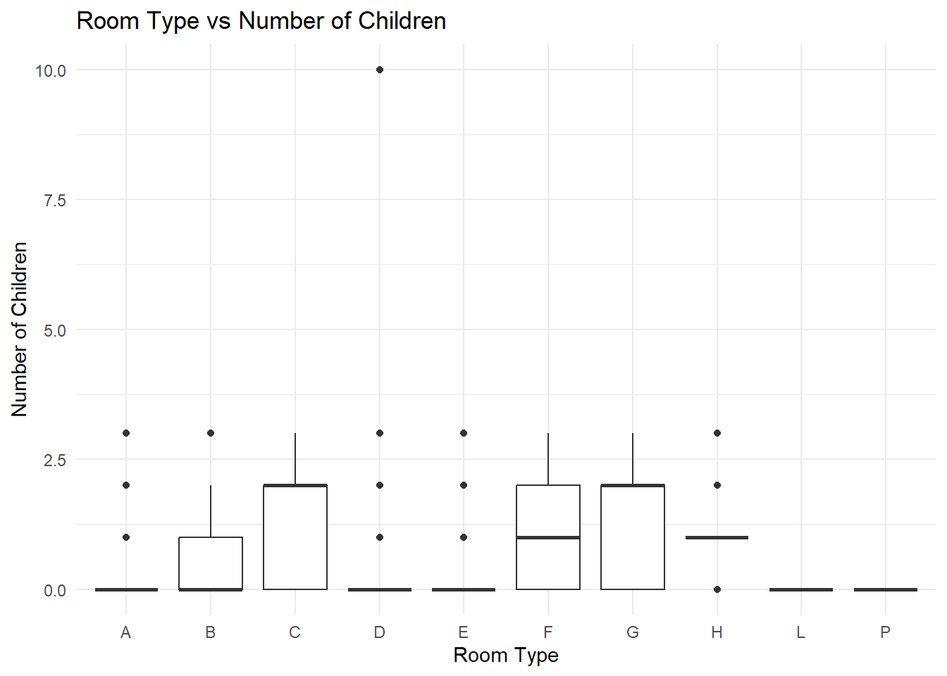
# Create a box plot to visualize the relationship between room type and number of babies
data %>%
ggplot(aes(x = reserved_room_type, y = babies)) +
geom_boxplot() +
labs(x = "Room Type", y = "Number of Babies",
title = "Room Type vs Number of Babies") +
theme_minimal()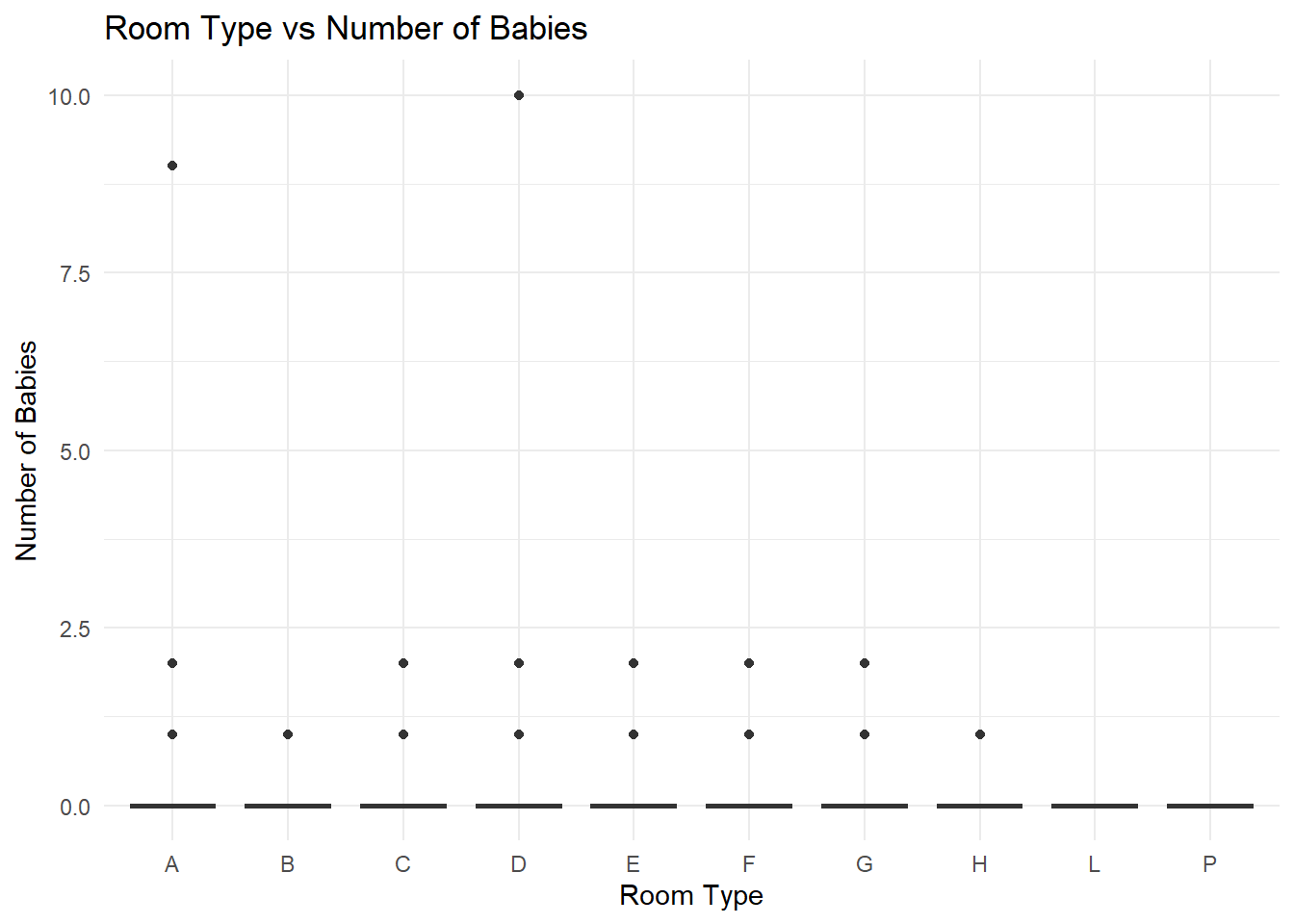
Based on the data, room type “A” is the most booked (87,500) suggesting high popularity, likely due to factors such as price, size, or amenities. Room type “D” is the second most favored (20,000 bookings). Room types “E” to “L” have fewer bookings, indicating less popularity. The least preferred are “P” and “L” with 1,000 bookings each, possibly due to higher pricing or limited availability. This data can guide the hotel’s strategic decisions, such as pricing adjustments, renovations, or marketing promotions, to enhance the attractiveness of less popular rooms and optimize the usage of the most popular ones. To get a fuller understanding, further analysis involving customer reviews, room prices, and room availability would be beneficial.
Firstly, we created a box plot for the relationship between room type and the number of adults. The x-axis represents different room types and the y-axis indicates the number of adults. For room type ‘A’, there are 40 individual points, while the range of 20-40 houses two points. The box plots for room types ‘B’, ‘C’, ‘D’, ‘E’, ‘F’, ‘G’, ‘H’, ‘L’, ‘P’ have medians between 0 and 3, and the boxes appear compressed, indicating a lower variance in the number of adults.
Similarly, we crafted a box plot to visualize the correlation between room type and the number of children. The boxes for ‘B’, ‘C’, ‘F’, and ‘G’ types appear larger, suggesting a larger variance in the number of children for these room types. However, the median for room types ‘A’, ‘B’, ‘C’, ‘D’, ‘E’, ‘F’, ‘G’, ‘H’, ‘L’, ‘P’ remains between 0 and 3.
Finally, a box plot was created to demonstrate the relationship between room type and the number of babies. Room types ‘A’, ‘B’, ‘C’, ‘D’, ‘E’, ‘F’, ‘G’, ‘H’ each have two points ranging from 0 to 2.5, whereas ‘L’ and ‘P’ have no babies. The boxes for all room types are quite flat, indicating a lower variance in the number of babies.
# Cancellations by lead time
ggplot(data, aes(x = lead_time)) +
geom_histogram(aes(fill = as.factor(is_canceled)), bins = 30, position = "fill") +
labs(x = "Lead Time (days)", y = "Proportion", fill = "Cancellation Status",
title = "Cancellation Rates by Lead Time") +
theme_minimal()Warning: Removed 4 rows containing missing values (`geom_bar()`).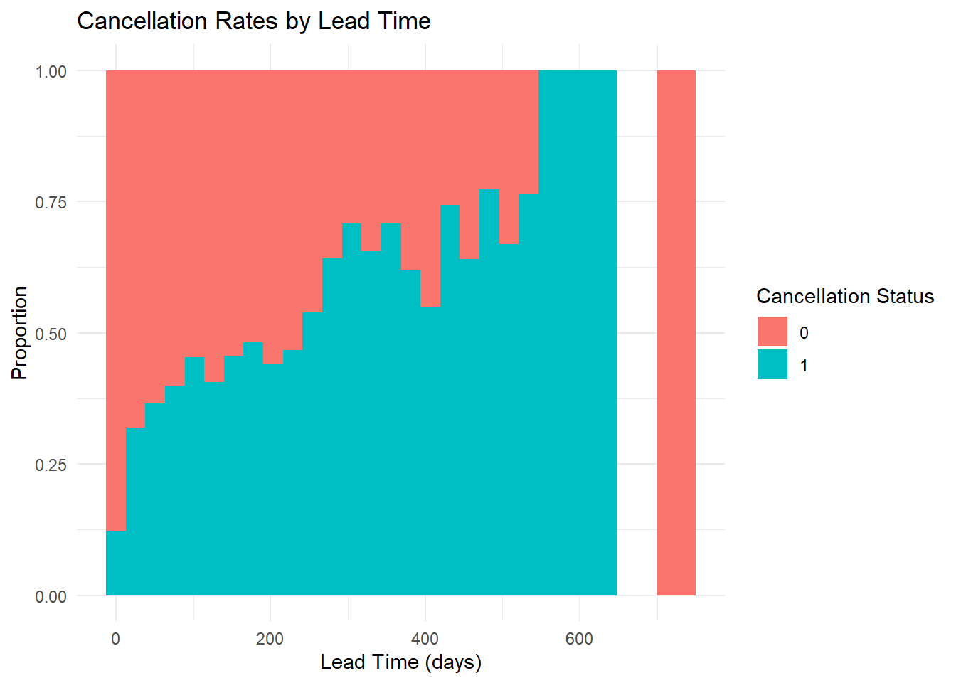
# Cancellations by room type
ggplot(data, aes(x = reserved_room_type)) +
geom_bar(aes(fill = as.factor(is_canceled)), position = "fill") +
labs(x = "Room Type", y = "Proportion", fill = "Cancellation Status",
title = "Cancellation Rates by Room Type") +
theme_minimal()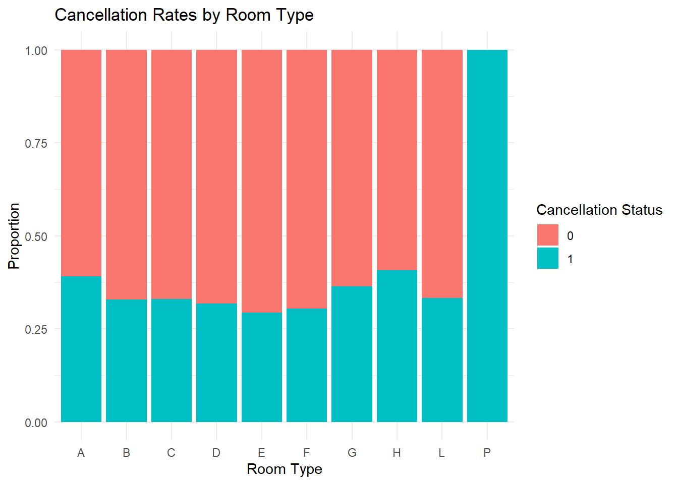
# Cancellations by repeated guest status
ggplot(data, aes(x = as.factor(is_repeated_guest))) +
geom_bar(aes(fill = as.factor(is_canceled)), position = "fill") +
labs(x = "Repeated Guest (0 = No, 1 = Yes)", y = "Proportion", fill = "Cancellation Status",
title = "Cancellation Rates by Repeated Guest Status") +
theme_minimal()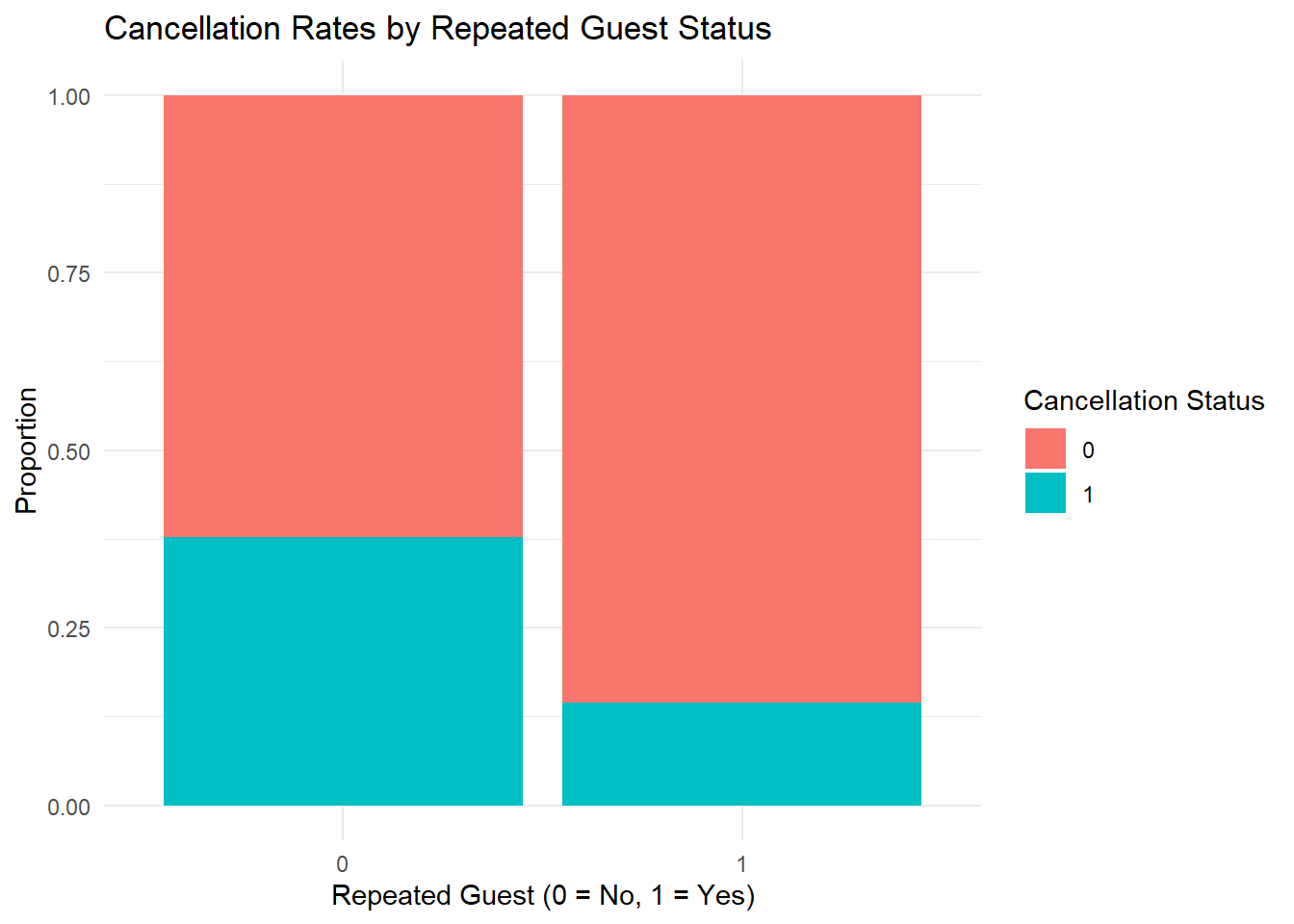
Using the ggplot2 package in R, we have created three insightful visualizations to explore cancellation patterns.
The first graph, titled “Cancellation Rates by Lead Time,” is a histogram showcasing the proportion of cancellations over a lead time range of 0 to 600 days. A clear trend surfaces that the cancellation rate escalates as lead time increases, suggesting that longer waits between booking and staying might lead to a higher likelihood of cancellation.
In the second plot, “Cancellation Rates by Room Type,” we delve into the relationship between room types and cancellation rates. Most room types (A through L) demonstrate a consistent cancellation rate hovering around 40%, barring Room P which startlingly exhibits a 100% cancellation rate. This points to potential issues specific to Room P that may need to be addressed.
The final chart, “Cancellation Rates by Repeated Guest Status,” compares the cancellation rates between new guests (labelled as 0) and returning guests (labelled as 1). Intriguingly, new guests exhibit a significantly higher cancellation rate of approximately 35%, as compared to the merely 12.5% of recurring guests, hinting at the reliability of repeated guests and the need for customer retention strategies.
model <- glm(is_canceled ~ lead_time + reserved_room_type + is_repeated_guest, data = data, family = binomial)
summary(model)
Call:
glm(formula = is_canceled ~ lead_time + reserved_room_type +
is_repeated_guest, family = binomial, data = data)
Coefficients:
Estimate Std. Error z value Pr(>|z|)
(Intercept) -1.067e+00 1.034e-02 -103.194 < 2e-16 ***
lead_time 5.663e-03 6.207e-05 91.227 < 2e-16 ***
reserved_room_typeB -3.244e-01 6.638e-02 -4.888 1.02e-06 ***
reserved_room_typeC -1.000e-01 7.188e-02 -1.392 0.164073
reserved_room_typeD -2.065e-01 1.756e-02 -11.763 < 2e-16 ***
reserved_room_typeE -3.550e-01 2.899e-02 -12.246 < 2e-16 ***
reserved_room_typeF -1.633e-01 4.201e-02 -3.886 0.000102 ***
reserved_room_typeG 5.615e-02 4.744e-02 1.183 0.236619
reserved_room_typeH 2.545e-01 8.609e-02 2.956 0.003119 **
reserved_room_typeL 3.736e-01 8.661e-01 0.431 0.666180
reserved_room_typeP 1.163e+01 3.449e+01 0.337 0.735887
is_repeated_guest -9.088e-01 4.765e-02 -19.073 < 2e-16 ***
---
Signif. codes: 0 '***' 0.001 '**' 0.01 '*' 0.05 '.' 0.1 ' ' 1
(Dispersion parameter for binomial family taken to be 1)
Null deviance: 157398 on 119389 degrees of freedom
Residual deviance: 146403 on 119378 degrees of freedom
AIC: 146427
Number of Fisher Scoring iterations: 9This output comes from a logistic regression model. It’s a statistical model we use when we want to predict something binary - in this case, whether a hotel booking was cancelled (1) or not (0).
The table you see lists a bunch of different factors that might affect the chance of a booking being cancelled.
First, look at the Estimate column. The values here, like 5.663e-03 for lead_time, represent how much we expect the log-odds of a cancellation to change when the factor increases by one unit. So, a longer lead time (time between booking and arrival) seems to slightly increase the chance of cancellation.
Then, check out the Pr(>|z|) column. This one’s all about how confident we are in these estimates. Smaller numbers here mean we’re pretty confident - like with lead_time, reserved_room_typeD, reserved_room_typeE, and is_repeated_guest. The stars in the rightmost column are another way of showing this - three stars mean we’re really confident.
But notice reserved_room_typeP and reserved_room_typeL? The big values in Pr(>|z|) (like 0.735887 and 0.666180) and lack of stars mean we’re not confident at all in these estimates.
Finally, at the very bottom, Null deviance and Residual deviance measure how well our model is doing. The smaller these numbers are, the better.
# Histogram of special requests frequency
ggplot(data, aes(x = total_of_special_requests)) +
geom_histogram(binwidth = 1, color = "black", fill = "skyblue") +
labs(x = "Number of Special Requests", y = "Count",
title = "Histogram of Special Requests Frequency") +
theme_minimal()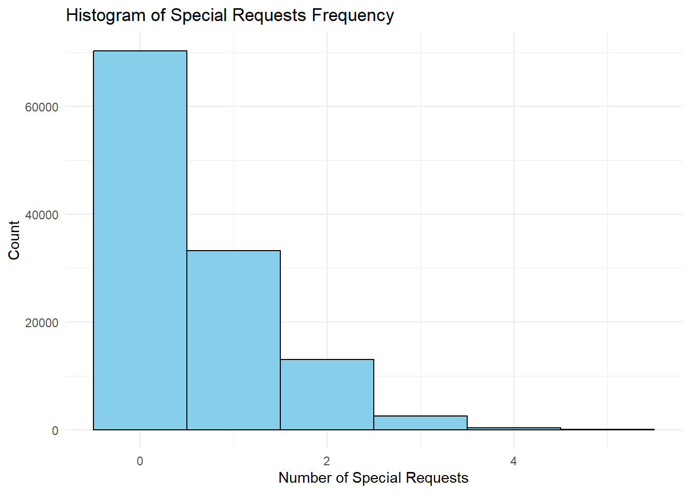
# Bar plot of cancellation rates by special requests
ggplot(data, aes(x = as.factor(total_of_special_requests), fill = as.factor(is_canceled))) +
geom_bar(position = "fill") +
scale_fill_discrete(name = "Cancellation Status", labels = c("Not Canceled", "Canceled")) +
labs(x = "Number of Special Requests", y = "Proportion",
title = "Cancellation Rates by Special Requests") +
theme_minimal()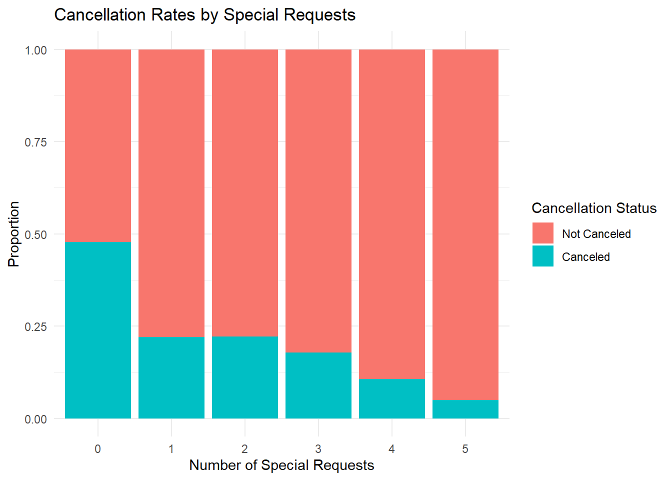
The histogram of special requests frequency indicates that the majority of customers do not have any special requests, accounting for approximately 70,100 of the total. As the number of special requests increases, the number of customers making these requests decreases substantially. For instance, only a small number of customers (33123) make one special request, with even fewer making two (13456), three (2001), or four (102) special requests. An extremely small number of customers make five special requests (only 2 customers).
The bar plot of cancellation rates by special requests reveals some interesting trends. For customers making no special requests, about 48% of their bookings are canceled. Interestingly, the cancellation rate declines as the number of special requests increases. For customers making one or two special requests, the cancellation rate is 24%, which further drops to 22% for those making three requests, 11.2% for four requests, and remarkably low at 5% for five requests.
In conclusion, most customers do not make special requests. However, those who do make special requests are less likely to cancel their bookings. This suggests that customers who take the time to customize their bookings with special requests are more committed to their stay.
# Scatter plot of ADR by the time of year
data %>%
mutate(month = lubridate::month(arrival_date, label = TRUE)) %>%
ggplot(aes(x = month, y = adr)) +
geom_point() +
labs(x = "Month", y = "Average Daily Rate (ADR)",
title = "ADR by Month") +
theme_minimal()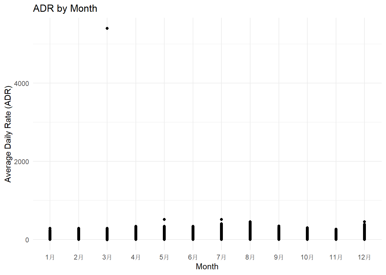
# Box plot of ADR by room type
data %>%
ggplot(aes(x = reserved_room_type, y = adr)) +
geom_boxplot() +
labs(x = "Room Type", y = "Average Daily Rate (ADR)",
title = "ADR by Room Type") +
theme_minimal()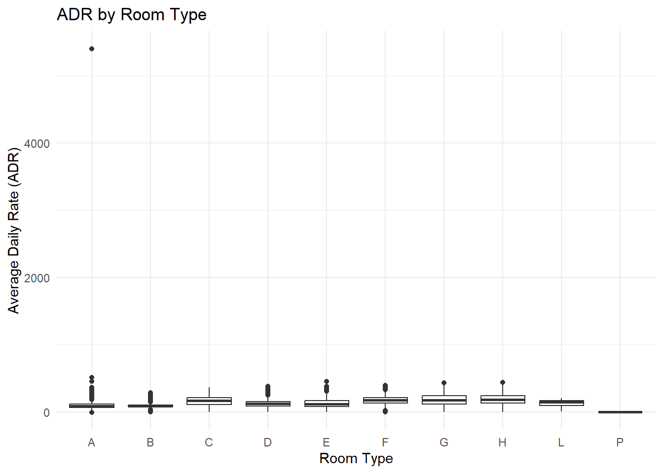
Looking at our data visualizations, we can see a definite pattern in pricing strategies. The price, also known as Average Daily Rate (ADR), does appear to vary based on the time of year and room type.
Starting with the scatter plot, it indicates that there is a monthly variation in ADR. Certain months appear to have a higher ADR than others, suggesting a potential influence of seasonality on hotel pricing. This could be due to a variety of factors, such as increased demand during holiday seasons or local events taking place.
The box plot displaying ADR by room type reveals a clear stratification of pricing. Each room type has a distinct price range, likely reflecting the different amenities, space, and comfort levels associated with each room.
So, it seems that the time of the year and the type of room are key factors influencing these pricing strategies. However, remember that these two factors are part of a larger, more complex pricing strategy which could also be influenced by factors like market demand, competitive pricing, local events, and economic conditions.
Our analysis focused on exploring various aspects of hotel data using visualizations as the primary approach, with statistics playing a supporting role. The goal was to uncover patterns, insights, and meaningful information rather than solely aiming for statistically significant results.
For booking patterns, we identified the busiest months for hotels and examined the relationship between booking numbers and lead time. This information can help with resource allocation and planning.
Regarding guest preferences, we investigated the popularity of different room types and their correlation with variables such as the number of adults, children, and babies in the party. Visualizing these relationships provided insights into guest preferences and potential influencing factors.
Cancellations were another area of interest. We analyzed cancellation patterns based on factors like lead time, room type, and repeated guest status. Visualizations helped us understand the relationship between these factors and cancellation rates, contributing to effective cancellation management and booking strategies.
We also explored special requests made by customers and their impact on cancellation likelihood. By visualizing the frequency of special requests and their correlation with cancellations, we gained insights into customer preferences and their influence on booking outcomes.
Lastly, we examined pricing strategies by investigating the variation in Average Daily Rate (ADR) based on the time of year and room type. Visualizations allowed us to identify potential pricing patterns, which can guide revenue management decisions.
Throughout the analysis, we prioritized storytelling and extracting meaningful insights from the data. While statistics were utilized to support our findings, the main focus was on presenting actionable insights and recommendations for the hotel industry.
Throughout the process of analyzing the hotel data and creating visualizations, we gained valuable insights and learned important lessons. We discovered the power of visualizations in uncovering patterns and trends within the data, allowing us to tell a compelling story and extract meaningful information. By focusing on visualizations and utilizing statistics as a supportive tool, we were able to explore the data in a comprehensive and accessible manner.
However, it is important to acknowledge the limitations of our dataset. While it provided us with valuable information about booking patterns, guest preferences, cancellations, special requests, and pricing strategies, there are still questions that remain unanswered. For example, our dataset did not include information about specific demographic factors of the guests or the specific reasons behind cancellations. Exploring these aspects could provide further insights into customer behavior and preferences.
In the process of putting together this project, we learned the importance of data exploration, visualization, and storytelling. We discovered that visualizations are a powerful tool for conveying complex information in a clear and concise manner. Additionally, we recognized the significance of identifying meaningful patterns and extracting actionable insights that can drive decision-making in the hotel industry.
Moving forward, there are several areas that could be explored in future research. Further analysis could delve into the impact of additional variables such as demographic factors, customer reviews, or marketing strategies on booking patterns and cancellations. Additionally, conducting surveys or interviews with guests could provide deeper insights into their preferences and motivations.
In conclusion, this project has demonstrated the value of visualizations and storytelling in data analysis. While our current findings have shed light on various aspects of the hotel industry, there is still much to explore and uncover. By continuing to leverage the power of visualizations and exploring additional variables, future research can contribute to a more comprehensive understanding of customer behavior and inform strategies for the hospitality sector.
Shrivas, S. (2022, October 19). Exploratory data analysis of Hotel Booking Demand - a case study. Medium. https://blog.devgenius.io/exploratory-data-analysis-of-hotel-booking-demand-a-case-study-4a27bff589ca
Wickham, H., & Grolemund, G. (2016). R for data science: Visualize, model, transform, tidy, and import data. https://r4ds.had.co.nz
R Core Team (2023). R: A Language and Environment for Statistical Computing. R Foundation for Statistical Computing, Vienna, Austria. https://www.R-project.org/.