Final Project: Food Security and Health Outcomes in U.S. Adults

An exploratory data analysis using the National Health and Nutrition Examination Survey (2017-2020)

Code

library(tidyverse)
library(here)
library(glue)
library(haven)
library(purrr)
library(ggplot2)
library(knitr)
library(kableExtra)

# get rid of summarize warnings
options(dplyr.summarise.inform = FALSE)
knitr::opts_chunk$set(echo = TRUE)

Background

The United States Department of Agriculture (USDA) defines household food security as having enough food so that all members of a household can live an active, healthy life (USDA, 2023). Conversely, food insecurity is characterized by being unable to attain enough food to meet the needs of all members of a household. In 2021, it was estimated that approximately 10.2% of households in the United States (13.5 million households) experienced some form of food insecurity in 2021.

Given the important role that food and nutrition play in health outcomes, research has been conducted to understand the relationship between food insecurity and metabolic health outcomes. Results have shown a significant relationship between food insecurity and several conditions, such as obesity (Hernandez, Reesor, & Murillo, 2017), insulin resistance (Bermudez-Millan et al., 2019), diabetes (Berkowitz et al., 2013), and cardiovascular diseases (Zierath et al., 2023).

C-reactive protein (CRP) is an inflammatory biomarker that is produced by the liver. Traditionally, it has been found to be elevated during instances of inflammation or infection. However, medical research has highlighted its ability to detect inflammation in blood vessels, and elevated CRP is now an established predictor for cardiovascular diseases (Harvard Health Publishing, 2017).

Given the association between food insecurity and increased incidence of metabolic conditions and heart disease, research has also focused on understanding the role that inflammatory biomarkers, such as CRP, could play in the onset of these conditions. Indeed, Gowda et al. (2012) found higher levels of CRP in U.S. adults experiencing food insecurity.

The goal of this project will be to replicate and expand upon the work of Gowda et al. (2012) by conducting an exploration of food security status, health outcomes, and inflammation in U.S. adults.

Data

This analysis utilizes data from the National Health and Nutrition Examination Survey (NHANES), an annual survey conducted by the National Center for Health Statistics (NCHS) that assesses the health and nutritional status of adults and children. Data is collected through comprehensive interviews and physical and laboratory examinations and is released on a biennial basis. Each year, approximately 5,000 Americans are chosen for inclusion in the survey, and the population sampled is designed to be representative of the United States population.

NHANES data is divided into five main categories:

Demographics Data: Demographic and socioeconomic information about study participants, such as country of birth, education level, gender, race, and age.

Dietary Data: Information about supplement-use and food/nutritional intake

Examination Data: Information that comes from a physical examination, such as blood pressure, anthropomorphic measures (e.g. weight), and oral health.

Laboratory Data: Information that comes from serum lab tests, such as blood lipids, liver proteins, and many others.

Questionnaire Data: Information that comes from an interview, including personal and family health history, medication use, physical activity, and many others.

Across these five categories, the full NHANES dataset includes approximately 94 tables. For this analysis, however, we will only use 12 tables from the Demographics, Examination, Laboratory, and Questionnaire categories. Due to the structure of NHANES data, all of the tables can be easily joined using the unique identification number for each subject.

The website for NHANES currently has data dating back to 1999 available to the public, but for this analysis, we will focus on the data collected from January 2017 to March 2020 (pre-pandemic data).

Import Data

NHANES data is publicly released as SAS transport files with the extension .XPT. Therefore, we will use the haven package to import the data.

Code

base_path <- here('posts', '_data', 'nhanes')
read_data_from_base <- function(path) {
  return(read_xpt(glue('{base_path}/{path}')))
}

# Questionnaire data
demo <- read_data_from_base('P_DEMO.XPT')
bp_chol <- read_data_from_base('P_BPQ.XPT')
depression <- read_data_from_base('P_DPQ.XPT')
diabetes <- read_data_from_base('P_DIQ.XPT')
exercise <- read_data_from_base('P_PAQ.XPT')
food_security <- read_data_from_base('P_FSQ.XPT')
# health_conditions <- read_data_from_base('P_MCQ.XPT')
insurance <- read_data_from_base('P_HIQ.XPT')
nutrition <- read_data_from_base('P_DBQ.XPT')

# Physical exam data
body <- read_data_from_base('P_BMX.XPT')

# Labs data
bc_count <- read_data_from_base('P_CBC.XPT')
cotinine <- read_data_from_base('P_COT.XPT')
crp <- read_data_from_base('P_HSCRP.XPT')

Data Cleaning

In order to use this data for exploratory data analysis, we must first clean the data. For each data table, we will:

1. Subset the data to only the columns needed for analysis
2. Rename columns to descriptive, easy-to-understand names
3. Recode values according to the documentation for the 2017-2020 NHANES cycle.
4. Cast columns to correct data types
5. Use mutate to create new columns that can be used in our analysis

A cleaned version of the data is shown for each table.

Code

# Functions

select_relevant_cols <- function(df, cols_list) {
  df <- df %>%
    select(all_of(cols_list))
  
  return(df)
}

Demographics Data

The Demographics dataset provides demographic information for all study participants (n = 15560). The raw dataset contains 29 columns, but we will limit the data to only include the following columns: identifier, age, gender, race/ethnicity, and income to poverty ratio.

Code

demo_cols <- c('SEQN', 'RIAGENDR', 'RIDAGEYR', 'RIDRETH3', 'INDFMPIR')
demo_clean <- demo %>% 
  select_relevant_cols(demo_cols) %>%
  rename(
    id = SEQN,
    gender = RIAGENDR,
    age = RIDAGEYR,
    race = RIDRETH3,
    income_poverty_ratio = INDFMPIR
  ) %>%
  mutate(
    gender = case_when(
      gender == 1 ~ 'M',
      gender == 2 ~ 'F',
      gender == '.' ~ NA
      ),
    gender = factor(gender, levels = c('M', 'F')),
    race = case_when(
      race == 1 | race == 2 ~ 'Hispanic',
      race == 3 ~ 'Non-Hispanic White',
      race == 4 ~ 'Non-Hispanic Black',
      race == 6 ~ 'Non-Hispanic Asian',
      race == 7 ~ 'Other Race',
      race == '.' ~ NA
    ),
    race = factor(race)
  )

demo_clean

Questionnaire Data

Blood Pressure and Cholesterol

The Blood Pressure and Cholesterol dataset contains information about each subject’s blood pressure and cholesterol status. The raw dataset contains data for a subset of NHANES participants (n = 10195) and consists of 11 columns. For our analyses, we will only use the columns that indicate if a subject has been told that they have high blood pressure or high cholesterol. For both conditions, the subject could respond with “Yes”, “No”, or not provide an answer.

Code

bp_chol_cols <- c('SEQN', 'BPQ020', 'BPQ080')
bp_chol_clean <- bp_chol %>%
  select_relevant_cols(bp_chol_cols) %>%
  rename(
    id = SEQN,
    high_bp = BPQ020,
    high_cholesterol = BPQ080
  ) %>%
  mutate(
    across(
      c(high_bp, high_cholesterol),
      ~case_when(.x == 1 ~ 'Yes',
                 .x == 2 ~ 'No',
                 .x %in% c(7, 9) ~ NA,
                 .x == '.' ~ NA)
    ),
    high_bp = factor(high_bp, levels = c('No', 'Yes')),
    high_cholesterol = factor(high_cholesterol, levels = c('No', 'Yes'))
  )

bp_chol_clean

Diabetes

The Diabetes dataset contains information about each subject’s diabetes status. The raw dataset contains data for a subset of NHANES participants (n = 14986) and consists of 28 columns. For our analyses, we will only use the columns that indicate if a subject has been told that they have diabetes or prediabetes. For diabetes, a subject could respond with “Yes”, “No”, “Borderline” or not provide a response. For prediabetes, a subject could respond with “Yes”, “No”, or not provide a response.

For more complete coverage of diabetes responses, the diabetes and prediabetes variables were combined into a single variable (diabetes_all) with three levels: “No”, “Yes”, or “Prediabetes”. (Note: “Borderline” diabetes responses were coded as “Prediabetes”.)

Code

diabetes_cols <- c('SEQN', 'DIQ010', 'DIQ160')
diabetes_clean <- diabetes %>%
  select_relevant_cols(diabetes_cols) %>%
  rename(
    id = SEQN,
    diabetes = DIQ010,
    prediabetes = DIQ160
  ) %>%
  mutate(
    diabetes = case_when(
      diabetes == 1 ~ 'Yes',
      diabetes == 2 ~ 'No',
      diabetes == 3 ~ 'Borderline',
      diabetes %in% c(7, 9) ~ NA,
      diabetes == '.' ~ NA
    ),
    # diabetes = factor(diabetes, levels = c('No', 'Borderline', 'Yes')),
    prediabetes = case_when(
      prediabetes == 1 ~ 'Yes',
      prediabetes == 2 ~ 'No',
      prediabetes %in% c(7, 9) ~ NA,
      prediabetes == '.' ~ NA
    ),
    diabetes_all = ifelse((diabetes == 'No' & prediabetes == 'Yes') | (diabetes == 'Borderline'), 'Prediabetes', diabetes),
    diabetes_all = factor(diabetes_all, levels = c('No', 'Prediabetes', 'Yes'))
  )

diabetes_clean

Diet Behavior and Nutrition

The Diet Behavior and Nutrition dataset provides information about a subject’s dietary habits and a self-evaluation of the healthiness of their diet. The raw dataset contains data for all NHANES participants (n = 15560) and consists of 46 columns. For our analyses, we will only use the columns that describe the healthiness of the diet and dietary patterns in terms of the frequency that types of meals are consumed (e.g. frozen food, fast food, ready-to-eat meals etc).

Code

nutrition_cols <- c('SEQN', 'DBQ700', 'DBD895', 'DBD900', 'DBD905', 'DBD910')
nutrition_clean <- nutrition %>%
  select_relevant_cols(nutrition_cols) %>%
  rename(
    id = SEQN,
    health_diet = DBQ700,
    n_meals_out = DBD895,
    n_meals_ff = DBD900,
    n_rte_meals = DBD905,
    n_frozen_meals = DBD910
  ) %>%
  mutate(
    health_diet = case_when(
      health_diet == 1 ~ 'Excellent', 
      health_diet == 2 ~ 'Very good', 
      health_diet == 3 ~ 'Good', 
      health_diet == 4 ~ 'Fair',
      health_diet == 5 ~ 'Poor',
      health_diet %in% c(7, 9) ~ NA,
      health_diet == '.' ~ NA
    ),
    health_diet = factor(health_diet, levels = c('Poor', 'Fair', 'Good', 'Very good', 'Excellent')),
    across(c('n_meals_out', 'n_meals_ff', 'n_rte_meals', 'n_frozen_meals'), ~ifelse((.x %in% c(5555, 7777, 9999)) | (.x == '.'), NA, .x))
  )

nutrition_clean

Exercise

The Physical Activity dataset contains data to describe the amount of physical activity that a subject gets on a daily and weekly basis. The raw dataset contains data for a subset of NHANES participants (n = 9693) and consists of 17 columns. Although the dataset contains information about physical activity performed through work, transportation, and recreation, for our analyses, we will only use the columns that describe a subject’s sedentary activity and recreational physical activity.

For vigorous and moderate recreational activity, a “Yes” response indicates at least 10 minutes of exercise per week. Sedentary activity indicates the amount of time per day that a subject spends sitting.

Code

exercise_cols <- c('SEQN', 'PAQ650', 'PAQ665', 'PAD680')
exercise_clean <- exercise %>%
   select_relevant_cols(exercise_cols) %>%
  rename(
    id = SEQN,
    vigorous_exercise = PAQ650,
    moderate_exercise = PAQ665,
    sedentary_minutes = PAD680
  ) %>%
  mutate(
    across(
      c(vigorous_exercise, moderate_exercise),
      ~case_when(.x == 1 ~ 'Yes', .x == 2 ~ 'No', .x %in% c(7, 9) ~ NA, .x == '.' ~ NA)
      ),
    vigorous_exercise = factor(vigorous_exercise, levels = c('Yes', 'No')),
    moderate_exercise = factor(moderate_exercise, levels = c('Yes', 'No')),
    sedentary_minutes = ifelse((sedentary_minutes %in% c(7777, 9999)) | (sedentary_minutes == '.'), NA, sedentary_minutes)
  )

exercise_clean

Food Security

The Food Security dataset contains information about individual and household access to food and food-related benefits. The raw dataset contains data for all NHANES participants (n = 15560) and consists of 20 columns. For our analysis, we will explore household food security and household access to food benefits (e.g. SNAP, food stamps) and emergency food (e.g. food banks, soup kitchens) in the last 12 months.

Code

food_security_cols <- c('SEQN', 'FSDHH', 'FSD151', 'FSQ012')
food_security_clean <- food_security %>%
  select_relevant_cols(food_security_cols) %>%
  rename(
    id = SEQN,
    hh_food_security = FSDHH,
    hh_emergency_food = FSD151,
    hh_fs_benefit = FSQ012
  ) %>%
  mutate(
    hh_food_security = case_when(
      hh_food_security == 1 ~ 'Full',
      hh_food_security == 2 ~ 'Marginal',
      hh_food_security == 3 ~ 'Low',
      hh_food_security == 4 ~ 'Very Low',
      hh_food_security == '.' ~ NA
    ),
    hh_food_security = factor(hh_food_security, levels = c('Full', 'Marginal', 'Low', 'Very Low')),
    across(c(hh_emergency_food, hh_fs_benefit), 
           ~case_when(.x == 1 ~ T,
                      .x == 2 ~ F,
                      .x %in% c(7, 9) ~ NA,
                      .x == '.' ~ NA))
    )

food_security_clean

Mental Health Screener

To screen participants’ mental health, NHANES administers the Patient Health Questionnaire (PHQ). The PHQ contains 9 questions that assess the frequency of depressive symptoms over a two week period. For each question, the participant can indicate if they’ve experienced the symptom “Not at all”, “Several Days”, “More than half the days”, or “Nearly every day”, and points ranging from 0 to 3 are assigned according to the response. The scores on each question are summed to produce a final score that ranges from 0 to 27.

This dataset contains PHQ data for a subset of NHANES subjects (n = 8965) participants. For this analysis, we will only use the final score.

Code

q_cols <- colnames(depression %>% select(-DPQ100, -SEQN))
depression_clean <- depression %>%
  mutate(across(everything(), ~ifelse(. %in% c(7, 9), NA, .))) %>%
  mutate(across(everything(), ~ifelse(. == '.', NA, .))) %>%
  rowwise() %>%
  mutate(total_score = sum(across(all_of(q_cols)))) %>% # do not remove NA! 
  ungroup() %>%
  select(id = SEQN, total_score, -all_of(q_cols))

depression_clean

Insurance

The Health Insurance dataset contains information about individual health insurance coverage. The raw dataset contains data for all NHANES participants (n = 15560) and consists of 14 columns, including data for many types of health insurance (e.g. private, Medicare, Medicaid). For our analysis, we will limit our data to the column that indicates if a subject is covered by any type of health insurance.

Code

insurance_cols <- c('SEQN', 'HIQ011')
insurance_clean <- insurance %>%
  select_relevant_cols(insurance_cols) %>%
  rename(
    id = SEQN,
    has_med_insurance = HIQ011
    ) %>% 
  mutate(
    has_med_insurance = case_when(
      has_med_insurance == 1 ~ 'Yes',
      has_med_insurance == 2 ~ 'No',
      has_med_insurance %in% c(7, 9) ~ NA,
      has_med_insurance == '.' ~ NA),
    has_med_insurance = factor(has_med_insurance, levels = c('No', 'Yes'))
  )

insurance_clean

Physical Examination Data

Body Measures

The Body Measures dataset provides information about a subject’s build. The raw dataset contains data for all NHANES participants (n = 14300) and consists of 22 columns. For our analysis, we will utilize the variables related to BMI, waist circumference, and hip circumference. Because the waist-to-hip ratio (WHR) can be an indicator of abdominal obesity, we will engineer this feature by dividing the waist circumference by the hip circumference.

To more easily interpret BMI and waist-to-hip ratio, we will also engineer two features to indicate health risk:

1. BMI Classification

• Underweight (BMI < 18.5)
• Normal Weight (18.5 \(\leq\) BMI \(\leq\) 24.9)
• Overweight (25 \(\leq\) BMI \(\leq\) 29.9)
• Obese (BMI > 30)

2. Waist-to-hip Ratio Risk Class (from Burgess, 2017)

• Low Risk: (WHR \(\leq\) 0.8 for women; WHR \(\leq\) 0.95 for men)
• Moderate Risk: (0.81 \(\leq\) WHR \(\leq\) 0.85 for women; 0.96 \(\leq\) WHR \(\leq\) 0.99 for men)
• High Risk (WHR \(\geq\) 0.86 for women; WHR \(\geq\) 1.0 for men)

Code

body_cols <- c('SEQN', 'BMXBMI', 'BMXWAIST', 'BMXHIP')
body_clean <- body %>%
  select_relevant_cols(body_cols) %>%
  mutate(across(body_cols[body_cols != 'SEQN'], ~ifelse(.x == '.', NA, .x))) %>%
  rename(
    id = SEQN,
    bmi = BMXBMI,
    waist_circ = BMXWAIST,
    hip_circ = BMXHIP
  ) %>%
  mutate(waist_hip_ratio = round(waist_circ/hip_circ, 2)) %>%
  # add gender col for interpretation of waist-hip-ratio
  left_join(demo_clean %>% select(id, gender), by = 'id') %>%
  # add cols for interpretability
  mutate(
    bmi_class = case_when(
    bmi < 18.5 ~ 'Underweight',
    bmi >= 18.5 & bmi <= 24.9 ~ 'Normal',
    bmi >= 25.0 & bmi <= 29.9 ~ 'Overweight',
    bmi >= 30 ~ 'Obese'
    ),
    bmi_class = factor(bmi_class, levels = c('Underweight', 'Normal', 'Overweight', 'Obese')),
    whr_risk_class = case_when(
      waist_hip_ratio <= 0.8 & gender == 'F' ~ 'Low',
      waist_hip_ratio <= 0.95 & gender == 'M' ~ 'Low',
      waist_hip_ratio >= 0.81 &  waist_hip_ratio <= 0.85 & gender == 'F' ~ 'Moderate',
      waist_hip_ratio >= 0.96 &  waist_hip_ratio <= 0.99 & gender == 'M' ~ 'Moderate',
      waist_hip_ratio >= 0.86 & gender == 'F' ~ 'High',
      waist_hip_ratio >= 1.0 & gender == 'M' ~ 'High',
    ),
    whr_risk_class = factor(whr_risk_class, levels = c('Low', 'Moderate', 'High'))
  ) %>%
  select(-waist_circ, -hip_circ, -gender)

body_clean

Laboratory Data

Blood Cell Count

The Complete Blood Count dataset provides a count of blood cells, including red blood cells, white blood cells, and platelets, as well as other details. The raw dataset contains data for a subset of NHANES participants (n = 13772) and consists of 22 columns. For our analysis, we will only be interested in White Blood Cells counts, and we will engineer a feature to indicate if a subject has elevated white blood cells (cell count > 11,000 cells/microliter). Elevated white blood cells could be indicative of infection or a more serious health condition and could impact analyses of other lab variables, such as CRP.

Code

bc_count_cols <- c('SEQN', 'LBXWBCSI')
bc_count_clean <- bc_count %>%
  select_relevant_cols(bc_count_cols) %>%
  rename(id = SEQN, wbc = LBXWBCSI) %>%
  # classify wbc count as elevated or not
  mutate(elevated_wbc = ifelse(wbc > 11, T, F))

bc_count_clean

Cotinine

Cotinine is a metabolite of nicotine, and its presence in blood can be used to measure an individual’s exposure to tobacco smoke or tobacco use. For this analysis, we use the Cotinine dataset to engineer features related to tobacco exposure and smoking status. We first use the criteria presented in Gowda, Hadley, & Aiello (2012) to classify tobacco exposure levels based on serum cotinine level. Next, we use the exposure classifications to classify a subject as a smoker or non-smoker.

The raw dataset contains data for a subset of NHANES subjects (n = 13027).

Code

cotinine_cols <- c('SEQN', 'LBXCOT', 'LBDCOTLC')
cotinine_clean <- cotinine %>%
  select_relevant_cols(cotinine_cols) %>%
    rename(
    id = SEQN,
    cot = LBXCOT,
    quality = LBDCOTLC
    ) %>%
  # if not detectable, count as 0 exposure
  mutate(
    cot = ifelse(quality == 1, 0, cot)
    ) %>%
  select(-quality) %>%
  mutate(
    tob_exp_level = case_when(
      cot == 0 ~ 'None',
      cot <= 15 ~ 'Secondhand',
      cot > 15 ~ 'Smoker',
      T ~ NA
    ),
    tob_exp_level = factor(tob_exp_level, levels = c('None', 'Secondhand', 'Smoker')),
    smoker = case_when(
      tob_exp_level %in% c('None', 'Secondhand') ~ 'Non-Smoker',
      tob_exp_level == 'Smoker' ~ 'Smoker',
      T ~ NA
      ),
    smoker = factor(smoker, levels = c('Non-Smoker', 'Smoker'))
  )

cotinine_clean

C-Reactive Protein

The high-sensitivity CRP dataset provides serum levels for C-Reactive Protein, an inflammatory biomarker. The raw dataset contains CRP measures for a subset of NHANES participants (n = 13772). There are three columns, corresponding to the participant ID, CRP measure (mg/L), and a quality metric. We will set any readings below the detection limit to NA.

Code

crp_cols <- c('SEQN', 'LBXHSCRP', 'LBDHRPLC')
crp_clean <- crp %>%
  select_relevant_cols(crp_cols) %>%
  rename(
    id = SEQN,
    crp_mgL = LBXHSCRP,
    quality = LBDHRPLC
    ) %>%
  # if not at detection limit, set crp to NA
  mutate(crp_mgL = ifelse(quality == 0, crp_mgL, NA)) %>%
  select(-quality)

crp_clean

Join Data

Finally, now that we have cleaned each individual dataset, we can use a left_join to combine our 12 datasets into a single dataset.

Code

df_to_join <- list(
  demo_clean,
  bp_chol_clean,
  depression_clean,
  diabetes_clean,
  exercise_clean,
  food_security_clean,
  insurance_clean,
  nutrition_clean,
  body_clean,
  bc_count_clean,
  cotinine_clean,
  crp_clean
)

# use purrr to join all data frames with one function call!
# https://stackoverflow.com/questions/32066402/how-to-perform-multiple-left-joins-using-dplyr-in-r
full_df <- reduce(df_to_join, left_join, by = 'id')

full_df

The joined data contains data for 15560 subjects.

Study Sample

Inclusion and Exclusion Criteria

We will require that all NHANES subjects be 18-64 years of age for inclusion in our analysis. We will exclude any subjects with a white blood cell count that is greater than 11,000 cells/ microliter of blood (as this could indicate an infection or more serious health condition, such as cancer). Additionally, we will exclude any subjects missing data in the columns needed for our primary analysis: gender, age, race, income-to-poverty ratio, medical insurance coverage, depression_score, health outcomes (high_bp, high_cholesterol, diabetes, bmi, waist_to_hip_ratio), household food security, smoker status, and C-reactive protein.

Code

core_cols <- c('gender', 'age', 'race', 'income_poverty_ratio', 'high_bp', 'high_cholesterol', 'diabetes_all', 'hh_food_security', 'bmi', 'waist_hip_ratio', 'has_med_insurance', 'smoker', 'crp_mgL', 'total_score')

sample <- full_df %>%
  filter(
    age > 18,
    age < 64,
    elevated_wbc != T
    ) %>%
  # https://stackoverflow.com/questions/33520854/filtering-data-frame-based-on-na-on-multiple-columns
  filter_at(vars(core_cols), all_vars(!is.na(.)))

sample

Following application of the inclusion and exclusion criteria, we are left with a final sample size of 4384 subjects.

Description of Sample

Prior to conducting an exploratory analysis to understand how health outcomes and inflammatory levels differ by food security status, we will begin by conducting a descriptive analysis of our study sample. This will help us discover demographic and/or lifestyle factors that differ between the food security groups and could aid in interpretation of later results.

Food Security

According to the USDA, food security can be classified according to four levels:

1. Full indicates that a household had no worries about food supply and had full access to adequate food.

2. Marginal indicates that a household had some worry about access to adequate food, but the quality, variety, and quantity of food intake was not substantially reduced.

3. Low indicates that a household experienced reduced quality and variety of food, but the quantity and regularity of food intake was not substantially reduced.

4. Very Low indicates that at least one household member had to reduce food intake due to insufficient resources to access adequate food.

The figure below shows the counts and percentages of subjects for each food security level in our sample of U.S. adults.

Code

n_total <- nrow(sample)

sample %>%
  group_by(hh_food_security) %>%
  summarize(count = n()) %>%
  mutate(proportion = count/n_total) %>%
  ggplot(aes(x=hh_food_security, y=count)) +
  geom_col(fill='#F8766D') +
  geom_text(aes(label = glue('{round(proportion * 100)}%')), vjust = -0.5) + 
  theme_minimal() +
  labs(
    title = 'Count of U.S. Adults by Food Security Level',
    subtitle = glue('n = {nrow(sample)}'),
    x = 'Food Security',
    y = 'Count'
  )

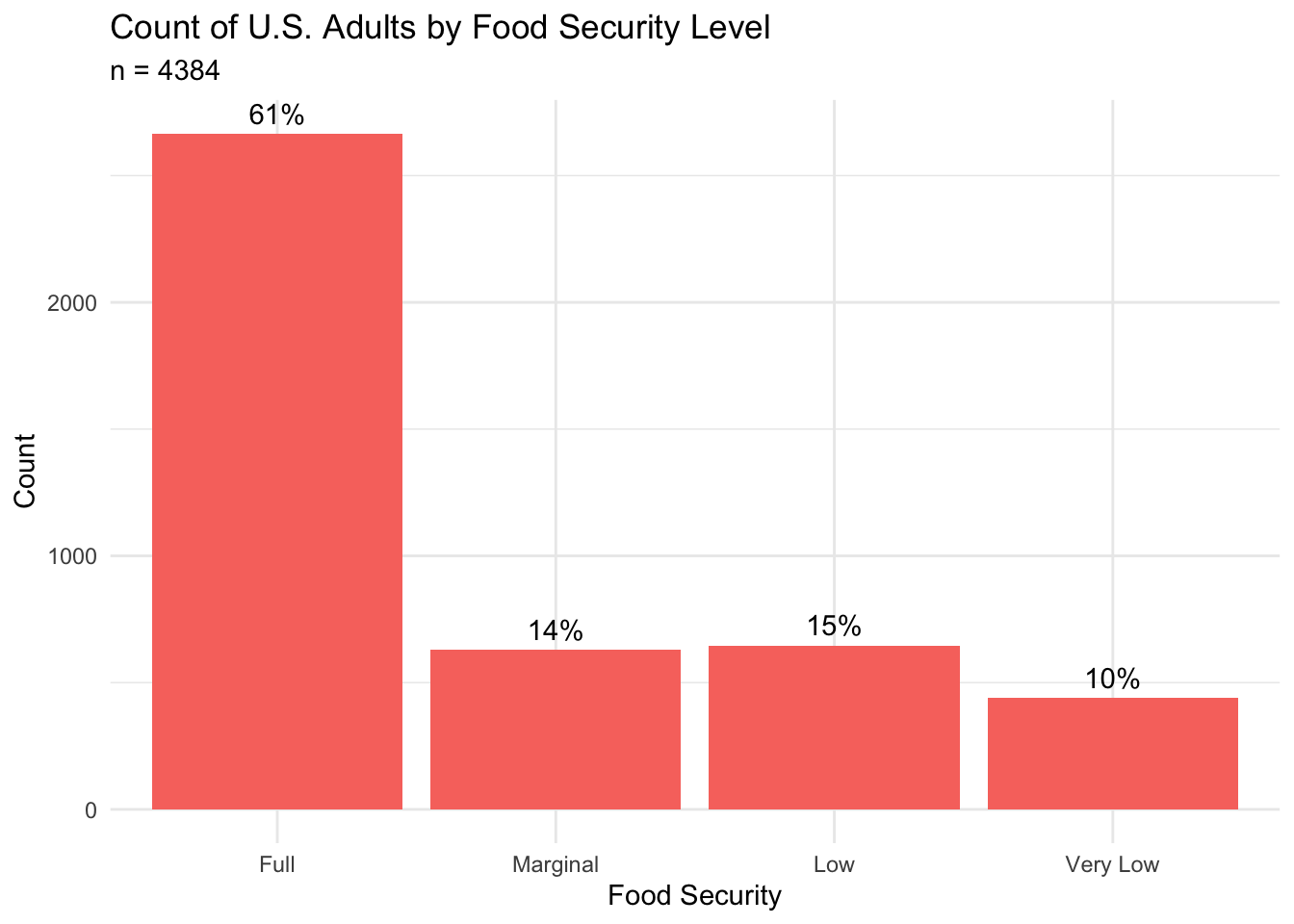
This figure shows that approximately 61% of subjects in our sample are fully food secure. However, almost 40% of subjects lived in a household that experienced some level of reduced food security, and approximately 10% lived in a household where at least one family member had decreased access to adequate food. The proportion of subjects experiencing low and very low food security in our sample (25%) is almost 2.5 times higher than the 10.2% reported by the USDA in 2021 (USDA, 2023). This suggests an overrepresentation of food-insecure subjects in our sample.

Age

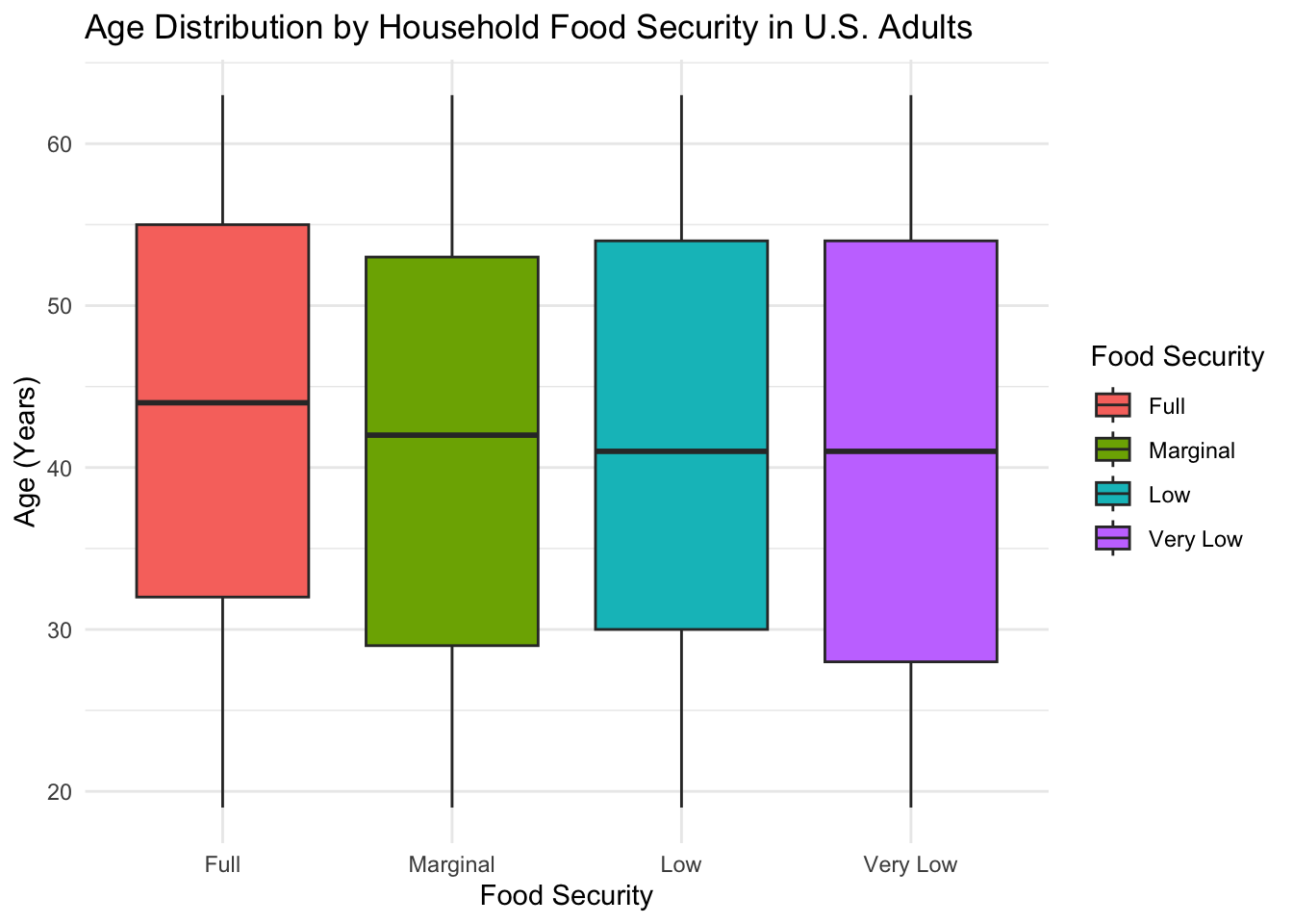
The age distribution for each food security group is shown below. As expected from our inclusion criteria, the age range across all groups spans 18-64 years of age.

Code

sample %>%
  ggplot(aes(x=hh_food_security, y=age, fill = hh_food_security)) +
  geom_boxplot() +
  theme_minimal() +
  labs(
    title = 'Age Distribution by Household Food Security in U.S. Adults',
    x = 'Food Security',
    y = 'Age (Years)',
    fill = 'Food Security'
    )

Code

medians <- sample %>% 
  group_by(hh_food_security) %>%
  summarize(median = median(age))

get_median_by_col_and_group <- function(column, food_security_group, df = sample) {
  medians <- df %>% 
    group_by(hh_food_security) %>%
    summarize(median = median(!!sym(column)))
  
  group_median <- medians %>%
    filter(hh_food_security == food_security_group) %>%
    pull(median)
 
  return(group_median) 
}

The box plots above show that the median age across all food security levels is older than 40 years of age. The group with “Full” food security has a slightly higher median age (age = 44) than the “Marginal” (age = 42), “Low” (age = 41), or “Very Low” (age = 41) food security groups. The variation in age appears to be highest for the “Very Low” food security group, as indicated by the length of the interquartile range.

If we examine the density of subjects by age and food security grouping (below), we can see that the median age for the fully food secure group is influenced by a high density of subjects between the ages of 50-60, indicating a large amount of older individuals that are fully food secure. Additionally, we see an interesting bimodal distribution within the “Very Low” food security group, which indicates a roughly equivalent amount of individuals experiencing food insecurity at both the younger (20-30) and older ages (50-55).

Code

sample %>%
  ggplot(aes(x=age, color = hh_food_security)) +
  geom_density() +
theme_minimal() +
labs(
  title = 'Age Density by Household Food Security in U.S. Adults',
  x = 'Age',
  y = 'Density',
  color = 'Food Security'
)

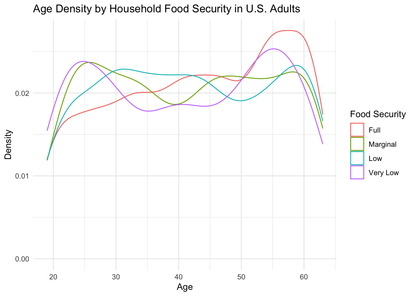
Given that health outcomes differ by age, the older age of the fully food-secure group could be an important factor to consider in later analyses.

Gender

Next, we explore differences in the binary gender composition of each food security group. The figure below shows the distribution (counts and percentages) of males and females in each group.

Code

counts_by_fs <- sample %>%
  group_by(hh_food_security) %>%
  summarize(total = n())

sample %>%
  group_by(gender, hh_food_security) %>%
  summarize(count = n()) %>%
  left_join(counts_by_fs, by = 'hh_food_security') %>%
  mutate(percent = count/total) %>%
  ggplot(aes(x = hh_food_security, y = count, fill = gender)) +
  geom_col(position = 'dodge') +
  geom_text(aes(label = glue('{round(percent * 100)}%'), group=gender), position = position_dodge(width = .9), vjust = -0.5) +
  theme_minimal() +
  labs(
  title = 'Gender Distribution by Food Security Level in U.S. Adults',
  subtitle = glue('n = {n_total}'),
  x = 'Food Security',
  y = 'Count',
  fill = 'Gender'
  )

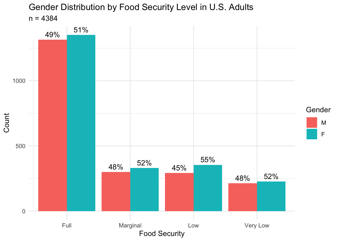
Across the entire sample, this figure shows that there are marginally more females (n = 2265; 51.7%) than males (n = 2119; 48.3%), and this trend remains when the data is subset by food security level.

When comparing food security groups, we see that the “Marginal” and “Very Low” food security groups (52% female) have a 1-percentage point higher proportion of females than the “Full” food security group (51% female), and the percentage of females in the “Low” food security group (55% female) is higher than the “Full” food security group by 4 percentage points. This observation suggests a slightly higher proportion of females in the groups experiencing reduced food insecurity. This is aligned with research that has found that, globally, women are more likely to be food-insecure than men (Broussard, 2019).

Race

We can also explore the composition of our sample by race and ethnic group. As a baseline, we begin by viewing the count and percentage of each racial and ethnic group for the entire sample.

Code

sample %>%
  group_by(race) %>%
  summarize(count = n()) %>%
  mutate(proportion = count/n_total) %>%
  ggplot(aes(x=race, y=count)) +
  geom_col(fill='#F8766D') +
  geom_text(aes(label = glue('{round(proportion * 100)}%'), hjust=-0.25)) + 
  ylim(0, 1600) + 
  theme_minimal() +
  labs(
    title = 'Distribution of U.S. Adults by Racial and Ethnic Group',
    subtitle = glue('n = {n_total}'),
    x = 'Race',
    y = 'Count'
  ) +
  coord_flip()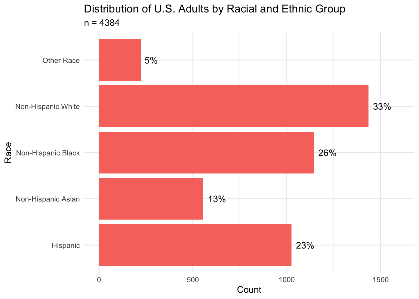

From this plot, we can see that the largest racial groups in our sample are Non-Hispanic White (33%), Non-Hispanic Black (26%), and Hispanic (23%).

The figure below shows the distribution of racial and ethnic groups for each food security level.

Code

sample %>%
  group_by(race, hh_food_security) %>%
  summarize(count = n()) %>%
  left_join(counts_by_fs, by = 'hh_food_security') %>%
  mutate(percent = count/total) %>%
  ggplot(aes(x = hh_food_security, y = percent, fill = race)) +
  geom_col(position = 'dodge') +
  theme_minimal() +
  scale_y_continuous(labels = scales::percent) +
  labs(
  title = 'Household Food Security by Race in U.S. Adults',
  x = 'Food Security',
  y = 'Percent',
  fill = 'Race'
  )

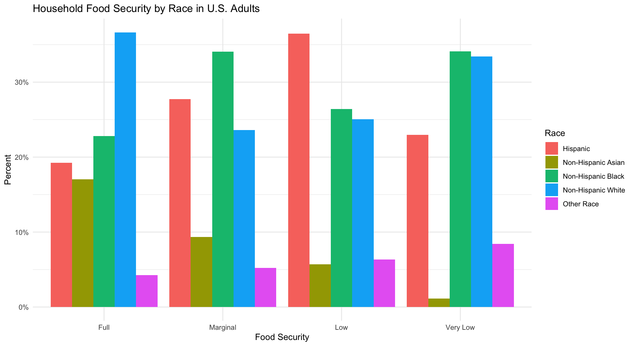
Across all food security levels, we see fairly good representation of Non-Hispanic White, Non-Hispanic Black, and Hispanic racial groups. Surprisingly, the Non-Hispanic Asian group has decreasing representation as the level of food-insecurity increases–a trend not seen in any of the other racial groups. This suggests less food insecurity in the Non-Hispanic Asian group.

If we compare the racial composition by food security group, we see that the largest individual racial group in the “Full” food security group is Non-Hispanic White (37%). However, there are also a substantial number of subjects belonging to the Non-Hispanic Black (23%), Hispanic (19%), and Non-Hispanic Asian (17%) groups. In the “Marginal” food security group, we see the largest number of subjects belonging to the Non-Hispanic Black (34%), Hispanic (28%), and Non-Hispanic White (24%) groups, and less representation of the Non-Hispanic Asian (9%) and Other (5%) racial groups. The “Low” food security group is composed of a large percentage of Hispanic (36%), Non-Hispanic Black (26%), and Non-Hispanic White (25%) subjects. The “Very Low” food security group has roughly equal percentages of Non-Hispanic Black and White subjects (33% and 34%, respectively) and slightly fewer Hispanic subjects (23%).

Overall, these results suggest representation of most races in each food security group. However, it appears that there are a higher percentage of Non-Hispanic White subjects in the “Full” food security group, a higher percentage of Non-Hispanic Black subjects in the “Marginal” food security group, and a higher percentage of Hispanic subjects in the “Low” food security group. The “Very Low” food security group has a higher percentage of Non-Hispanic Black and White subjects.

Smoking Status

Given that the risk for several metabolic health conditions, such as obesity, diabetes, and hypertension, can be exacerbated by cigarette smoking, for our future analyses, it will be important to understand any differences in smoking habits between the food security groups.

The figure below shows the counts and percentages of non-smokers and smokers for each group.

Code

sample %>%
  group_by(smoker, hh_food_security) %>%
  summarize(count = n()) %>%
  left_join(counts_by_fs, by = 'hh_food_security') %>%
  mutate(percent = count/total) %>%
  ggplot(aes(x = hh_food_security, y = count, fill = smoker)) +
  geom_col(position = 'dodge') +
  geom_text(aes(label = glue('{round(percent * 100)}%'), group=smoker), position = position_dodge(width = .9), vjust = -0.5) +
  theme_minimal() +
  labs(
  title = 'Distribution of Smoking Status by Food Security Level in U.S. Adults',
  subtitle = glue('n = {n_total}'),
  x = 'Food Security',
  y = 'Count',
  fill = 'Smoking Status'
  )

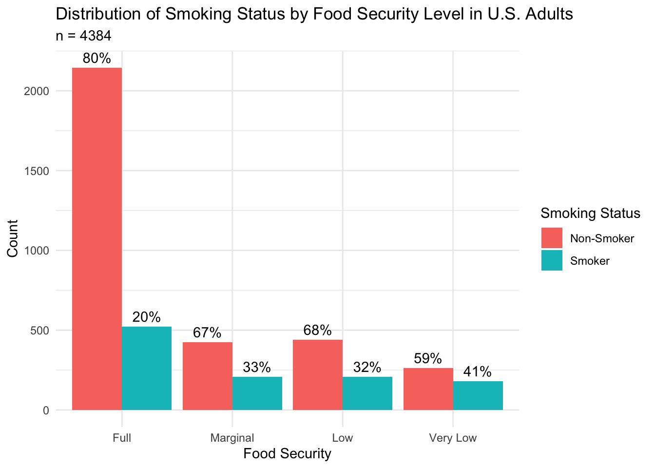
In this figure, we see that the “Full” food security group (80% non-smoker) contains a higher proportion of non-smokers than the “Marginal” (67% non-smoker), “Low” (68% non-smoker), and “Very Low” (59% non-smoker) food security groups. When interpreting differences in health outcomes by food security group, we should consider the influence that a higher proportion of smokers could have on our analyses of the groups experiencing reduced food security.

Income-to-Poverty Ratio

To help characterize our sample, we are also interested in understanding the socioeconomic status of each food security group. The income-to-poverty ratio is a metric that is computed by dividing the household’s annual income by the value of the poverty cut-off. A value less than 1 indicates an annual income that is below the poverty line, while a value that is greater than 1 indicates an annual income that is above the poverty line.

The figure below shows the distribution of the income to poverty ratio for each food security group.

Code

sample %>% 
  ggplot(aes(x=hh_food_security, y=income_poverty_ratio, fill = hh_food_security)) +
  geom_boxplot() +
  theme_minimal() +
  labs(
    title = 'Distribution of Income-to-Poverty Ratio by Household Food Security in U.S. Adults',
    x = 'Food Security',
    y = 'Income-to-Poverty Ratio',
    fill = 'Food Security'
  )

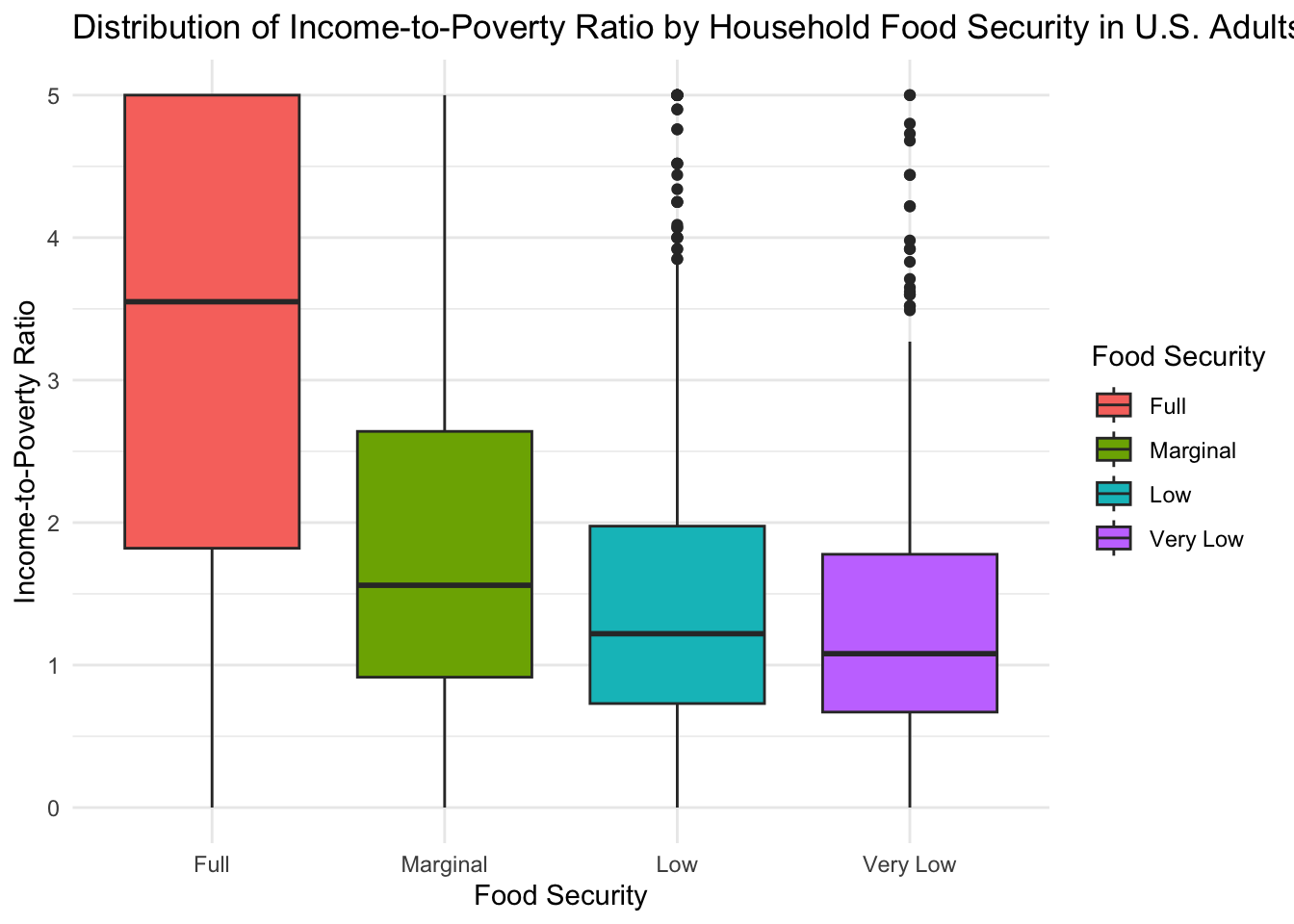
This figure shows a striking difference in the income-to-poverty ratio for different food security groups. The median income-to-poverty ratio for the group with “Full” food security (IPR = 3.55) was over twice as large as the highest median ratio for the “Marginal” (IPR = 1.56), “Low” (IPR = 1.22), and “Very Low” (IPR = 1.08) food security groups. Furthermore, the boxplot shows that the 25th percentile for the groups experiencing reduced food security is below an income-to-poverty ratio of 1, indicating that at least 25% of these subjects live below the poverty line.

Given that food security requires sufficient resources to access adequate food, these differences in socioeconomic standing are not surprising but are important to keep in mind when interpreting future results.

Health Insurance Coverage

Within the United States, where healthcare is known for being expensive, it is also important to understand the health insurance coverage of the subjects in our sample. The figure below shows the counts and percentages of subjects with insurance coverage for each food security group.

Code

sample %>%
  group_by(has_med_insurance, hh_food_security) %>%
  summarize(count = n()) %>%
  left_join(counts_by_fs, by = 'hh_food_security') %>%
  mutate(percent = count/total) %>%
  ggplot(aes(x = hh_food_security, y = count, fill = has_med_insurance)) +
  geom_col(position = 'dodge') +
  geom_text(aes(label = glue('{round(percent * 100)}%'), group=has_med_insurance), position = position_dodge(width = .9), vjust = -0.5) +
  theme_minimal() +
  labs(
  title = 'Distribution of Medical Insurance Coverage by Household Food Security in U.S. Adults',
  x = 'Food Security',
  y = 'Count',
  fill = 'Medical Insurance Coverage'
  )

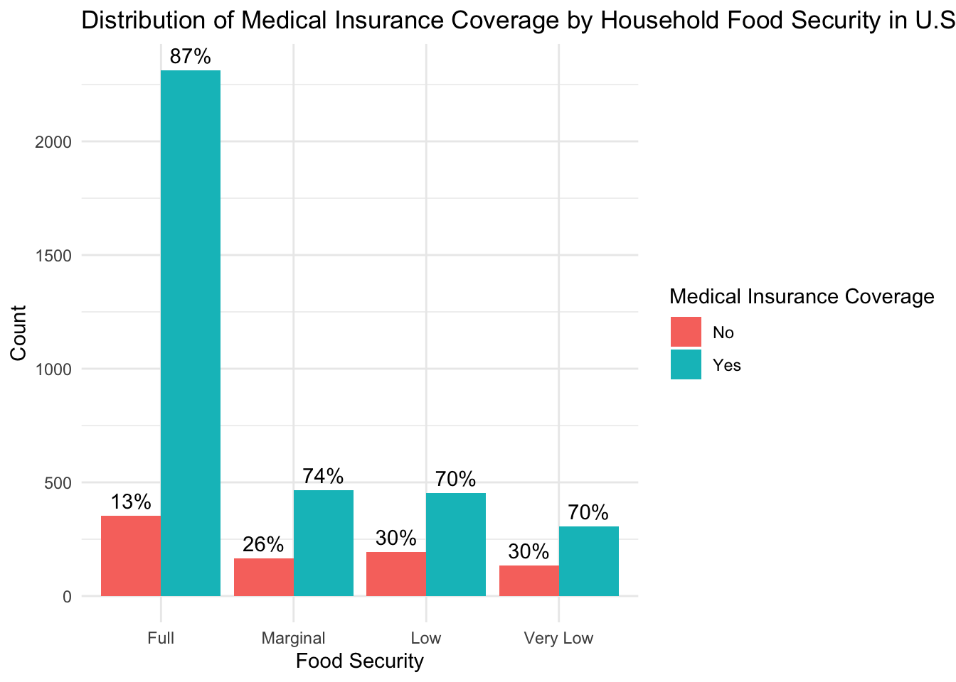
From this figure, we can see that, overall, there is good health insurance coverage across all food security groups; at least 70% of subjects in each group have access to health insurance. However, there is a 13 to 17 percentage point difference in coverage between the “Full” food security group and the groups experiencing reduced food security and a trend of decreasing insurance coverage as the level of food insecurity increases. Given that a lack of insurance might decrease healthcare-seeking behaviors, insurance coverage could be an important factor to consider when interpreting the results of our analyses.

Mental Health Status

Finally, as described above, the definition for each food security levels contains a statement about the level of “worry” that a subject feels about being able to secure adequate food. As such, in addition to the nutritional challenges posed by reduced access to food, it is likely that food insecurity could also serve as a psychological stressor that could potentially worsen a subject’s health. Unfortunately, the NHANES dataset does not contain a questionnaire to directly evaluate subjects’ stress levels or to understand subjects’ perceived stressors. Therefore, as a proxy for psychological stress, we will use the questionnaire that NHANES uses to assess subjects’ mental health status, the Patient Health Questionnaire (PHQ-9; Kroenke, Spitzer, & Williams, 2001). As described during data cleaning, this questionnaire provides a total score that can be used to interpret the level of depression a subject is feeling.

The scoring cut-offs for each depression severity class are as follows:

Code

scores <- c('0', '1-4', '5-9', '10-14', '15-19', '20-27')
names <- c('No Depression', 'Minimal Depression', 'Mild Depression', 'Moderate Depression', 'Moderate-Severe Depression', 'Severe Depression')
desc_table <- data.frame(Score = scores, Classification = names)

kbl(desc_table, booktabs = T) # %>% 

Score	Classification
0	No Depression
1-4	Minimal Depression
5-9	Mild Depression
10-14	Moderate Depression
15-19	Moderate-Severe Depression
20-27	Severe Depression

Code

#   kable_styling(latex_options = "striped")

The figure below shows the distribution of PHQ-9 scores for each food security level. The left boundary for each depression severity class is also shown.

Code

sample %>%
  ggplot() + 
  geom_density(aes(total_score, color = hh_food_security)) +
  geom_vline(aes(xintercept=1), linetype='dotted') +
  geom_text(aes(x=1, label="\nMinimal", y=0.288), angle=90) +
  geom_vline(aes(xintercept=5), linetype='dotted') +
  geom_text(aes(x=5, label="\nMild", y=0.298), angle=90) +
  geom_vline(aes(xintercept=10), linetype='dotted') +
  geom_text(aes(x=10, label="\nModerate", y=0.285), angle=90) +
  geom_vline(aes(xintercept=15), linetype='dotted') +
  geom_text(aes(x=15, label="\nModerate-Severe", y=0.265), angle=90) +
  geom_vline(aes(xintercept=20), linetype='dotted') +
  geom_text(aes(x=20, label="\nSevere", y=0.292), angle=90) +
  theme_minimal() +
  labs(
    title = 'Distribution of PHQ-9 Depression Score by Food Security Level in U.S. Adults',
    x = 'Depression Score',
    y = 'Density',
    color = 'Food Security'
  )

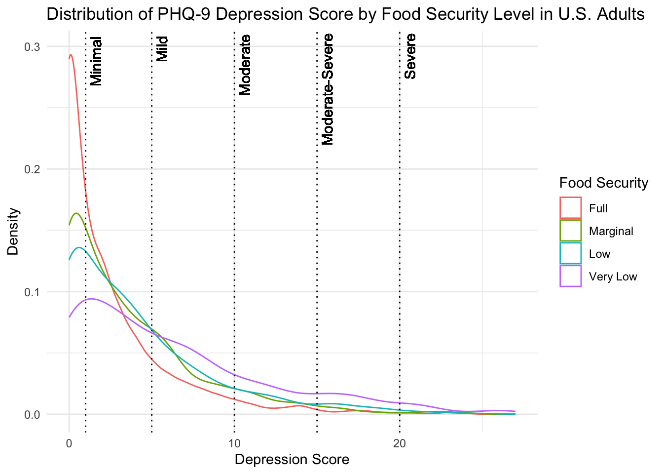
From this figure, we can see that a large proportion of a subjects in each food security group self-reported no depressive symptoms on the PHQ-9. If we compare levels of depression severity across the food security groups, however, we see that the “Full” food security group consistently has the lowest density of depression scores across most classifications of depression. This could indicate better mental health in this group of subjects or increased hesitancy to self-report symptoms. On the other hand, the group of subjects in the “Very Low” food security group show the highest density of subjects experiencing symptoms consistent with “Mild”, “Moderate”, “Moderate-Severe”, and “Severe” depression. This suggests poorer self-reported mental health in this group of subjects. However, due to the nature of the data, we are unable to directly attribute any differences in mental health status to access to adequate food.

The above analyses provided a thorough exploration of the demographic and lifestyle characteristics for each food security group in our sample.

Research Questions

Our goals for this exploratory data analysis will be to better understand health outcomes in our sample of U.S. adults.

The primary research questions that we will explore are:

1. Does the prevalence of metabolic health conditions, such as high blood pressure, high cholesterol, diabetes, and obesity, differ by food security levels in our sample of U.S. adults?

2. Do levels of inflammatory factors, such as C-reactive protein, differ by food security levels in our sample of U.S. adults? If so, could inflammatory factors help explain the relationship between food security and health outcomes?

Data Analysis

RQ 1: Food Security and Health Outcomes

As mentioned in the introduction to the project, many research studies that have explored health outcomes in food-insecure individuals have focused on metabolic conditions (conditions that are risk factors for cardiovascular diseases), such as obesity and diabetes. Therefore, for our analysis, we will also examine how the incidence of metabolic conditions differs by food security status.

Obesity

The first health outcome that we will explore is obesity, which is a condition that is characterized by an excess of body fat. Within our subset of NHANES data, there are two variables that can be used to diagnose obesity and interpret the health risks associated with differing levels of body fat. These variables are the Body Mass Index (BMI), which is a function of weight and height, and waist-to-hip ratio (WHR), which is a ratio of waist circumference to hip circumference.

Body Mass Index

The figure below displays the BMI distribution for each food security group.

Code

sample %>%
  ggplot(aes(x = hh_food_security, y = bmi, fill = hh_food_security)) +
  geom_boxplot() +
  theme_minimal() +
  labs(
    title = "BMI Distribution by Food Security Status in U.S. Adults",
    x = 'Food Security',
    y = 'BMI',
    fill = 'Food Security'
  )

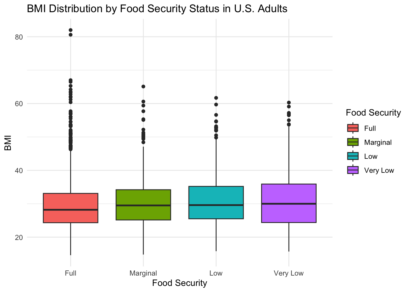
From this figure, we can see that the median BMI across all food security groups is greater than 25. This means means that approximately 50% of subjects in each food security group have a BMI that would be classified as overweight or higher. If we compare the distributions across food security groups, however, we see that the median BMI for the “Full” food security group (BMI = 28.2) is slightly lower than the median BMI for the “Marginal” (BMI = 29.5), “Low” (BMI = 29.6), and “Very Low” (BMI = 30) food security groups. Of the four food security groups, only the group experiencing the highest level of food insecurity has a BMI that would be classified as obese, suggesting a higher prevalence of obesity in this group.

The figure below presents the percentage of subjects in each food security group by BMI classification.

Code

counts_by_fs <- sample %>%
  group_by(hh_food_security) %>%
  summarize(total = n())

bmi_tally <- sample %>%
  group_by(bmi_class, hh_food_security) %>%
  summarize(count = n()) %>%
  left_join(counts_by_fs, by = 'hh_food_security') %>%
  mutate(percent = count/total)

bmi_tally %>%
  ggplot(aes(x = hh_food_security, y = percent, fill = bmi_class)) +
  geom_col(position='dodge') +
  theme_minimal() +
  scale_y_continuous(labels = scales::percent) +
  labs(
    title = 'BMI Classification by Food Security Group in U.S. Adults',
    x = 'Food Security',
    y = 'Percent',
    fill = 'BMI Classification'
    )

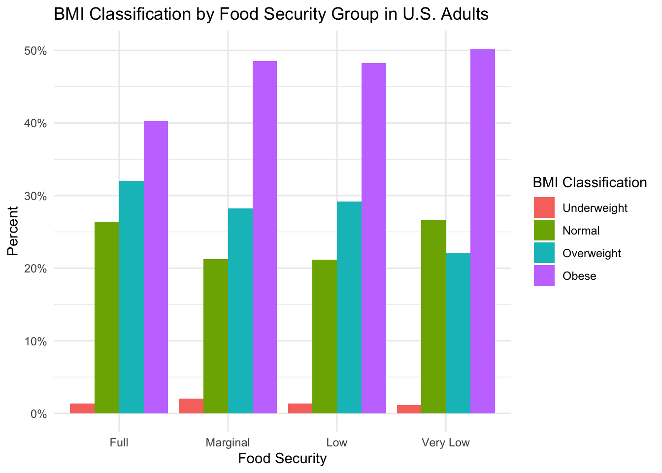
Perhaps somewhat surprising, this figure shows that, across all food security groups, the largest percentage of subjects have a BMI that falls in the “Obese” category–indicating a high incidence of adverse metabolic health across all groups. However, if the incidence of obesity in the fully food secure group is compared to the incidence of obesity in the groups experiencing some form of food insecurity, we see lower obesity incidence with “Full” food security. This suggests that, similar to the literature, food insecurity could be associated with higher rates of obesity in our sample (as determined by BMI).

Waist-to-Hip Ratio

As mentioned above, the waist-to-hip ratio (WHR) is another way to measure excess body fat and also provides a way to interpret the effect of differing body shapes on health risk. The figure below shows the distribution of WHR by food security group for our sample of U.S. adults.

Code

sample %>%
  ggplot(aes(x = hh_food_security, y = waist_hip_ratio, fill = hh_food_security)) +
  geom_boxplot() +
  theme_minimal() +
  labs(
    title = "Distribution of Waist-to-Hip Ratio (WHR) by Food Security Status in U.S. Adults",
    x = 'Food Security',
    y = 'WHR',
    fill = 'Food Security'
  )

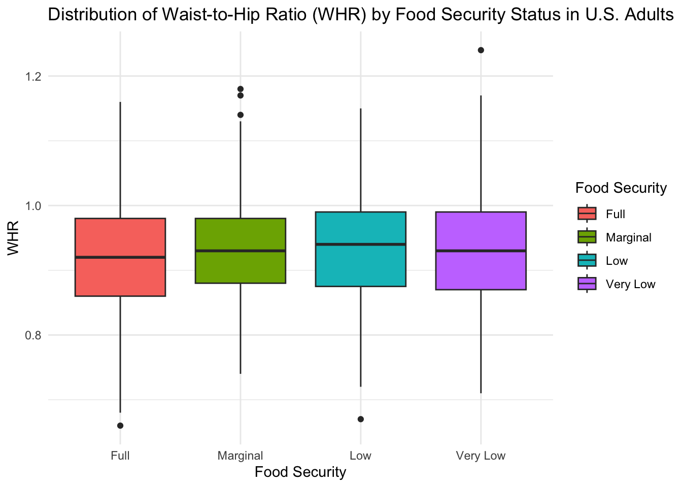
Using this figure, we see that the median WHR for the “Full” food security group (WHR = 0.92) is slightly lower than the median WHR for the “Marginal” (WHR = 0.93), “Low” (WHR = 0.94), and “Very Low” (WHR = 0.93) food security groups.

As described when cleaning the data, an individual’s WHR can also be used to assess cardiovascular risk. Below, we subset the data by food security group and show the percentage of subjects in each WHR risk class.

Code

counts_by_fs <- sample %>%
  group_by(hh_food_security) %>%
  summarize(total = n())

whr_tally <- sample %>%
  group_by(whr_risk_class, hh_food_security) %>%
  summarize(count = n()) %>%
  left_join(counts_by_fs, by = 'hh_food_security') %>%
  mutate(percent = count/total)

whr_tally %>%
  ggplot(aes(x = hh_food_security, y = percent, fill = whr_risk_class)) +
  geom_col(position='dodge') +
  theme_minimal() +
  scale_y_continuous(labels = scales::percent) +
  labs(
    title = 'Waist-to-Hip Ratio (WHR) Risk Class by Food Security Group in U.S. Adults',
    x = 'Food Security',
    y = 'Percent',
    fill = 'WHR Risk Class'
    )

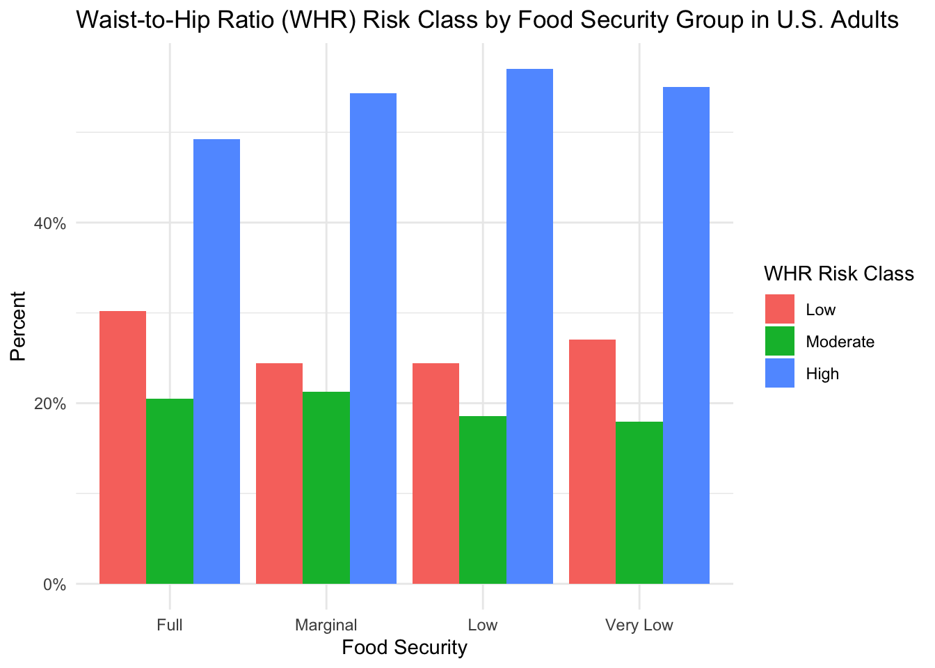
Upon reviewing the figure, it is immediately evident that the largest group of subjects in each food security group have a WHR that is considered high-risk for adverse health outcomes. Given that BMI and WHR can both be used to assess obesity and that we previously showed a high proportion of subjects with an obese BMI, this result is not surprising. When we compare the risk associated with WHR across the different food security groups, a similar trend to BMI also emerges. Compared to the “Marginal”, “Low”, and “Very Low” food security groups, we tend to see a higher percentage of subjects with a low-risk WHR and a slightly lower percentage of subjects with a high-risk WHR in the “Full” security group. Similar to the analyses with BMI, this suggests a larger percentage of subjects with an unhealthy WHR in groups experiencing reduced food security.

Combined, the results from the BMI and WHR analyses suggest an increased incidence of obesity in groups experiencing some form of food insecurity, and the analyses of the WHR further suggest an increased risk of future adverse outcomes in these groups.

Diabetes

In addition to obesity, another metabolic condition that we are interested in exploring is diabetes, a condition characterized by high blood sugar. Below, we subset the data by food security group and show the percentage of subjects in each group that have or have not been diagnosed with diabetes or prediabetes.

Code

plot_prop_by_condition <- function(df, condition_col, title_label, fill_label) {
  # get total counts for each food security group
  counts_by_fs <- df %>%
    group_by(hh_food_security) %>%
    summarize(total = n())

  # make the plot
  plt <- df %>%
    group_by(!!sym(condition_col), hh_food_security) %>%
    summarize(count = n()) %>%
    left_join(counts_by_fs, by = 'hh_food_security') %>%
    mutate(percent = count/total) %>%
    ggplot(aes(x = hh_food_security, y = percent, fill = !!sym(condition_col))) +
    geom_col(position='dodge') +
    theme_minimal() +
    scale_y_continuous(labels = scales::percent) +
    labs(
      title = title_label,
      x = 'Food Security',
      y = 'Percent',
      fill = fill_label
    )
  
  # return the plt
  return(plt)
}

plot_prop_by_condition(
  df = sample,
  condition_col = 'diabetes_all',
  title_label = 'Diabetes Classification by Food Security Group in U.S. Adults',
  fill_label = 'Diabetes'
)

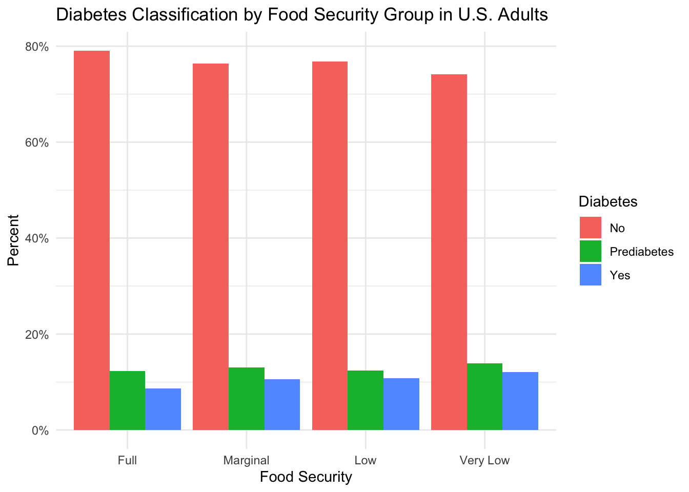
From the figure above, we can see that over 70% of subjects in each food security group have never been told by a doctor that they have diabetes. If we compare the data across the food security groups, however, we see that the percentage of subjects who have never been diagnosed with diabetes is slightly higher in the “Full” food security group compared to the subjects in groups experiencing a reduction in food security. Furthermore, compared to the “Full” food security group, we see that the percentage of subjects diagnosed with prediabetes and diabetes is slightly higher in the “Marginal” and “Low” food security groups. The largest difference in prediabetes and diabetes incidence occurs between the “Full” and “Very Low” food security groups, where prediabetes is higher in the “Very Low” food security group by approximately 2 percentage points and diabetes is higher by approximately 3 percentage points.

The results of this analysis suggest a small increase in the incidence of prediabetes and diabetes in groups experiencing some level of food insecurity.

High Blood Pressure

Another metabolic condition of interest is high blood pressure. Below, we see the proportion of subjects diagnosed with high blood pressure for each food security group.

Code

plot_prop_by_condition(
  df = sample,
  condition_col = 'high_bp',
  title_label = 'Blood Pressure Status by Food Security Group in U.S. Adults',
  fill_label = 'High Blood Pressure'
)

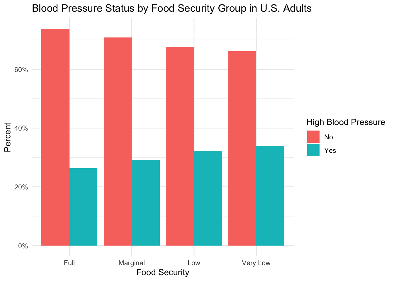
The figure above shows that the majority of subjects in each food security group have not been previously diagnosed with high blood pressure. However, when the data is compared across food security groups, we observe a trend towards increasing incidence in high blood pressure as the level of food security decreases. Indeed, the rate of high blood pressure by food security group is: “Full” (26%), “Marginal” (29%), “Low” (32%), and “Very Low” (33%).

The results of this analysis suggest a higher incidence of high blood pressure in groups experiencing reduced food security–especially groups classified as “Low” and “Very Low”.

High Cholesterol

Finally, we explore how the proportion of subjects who have been diagnosed with high cholesterol differs by food insecurity level.

Code

plot_prop_by_condition(
  df = sample,
  condition_col = 'high_cholesterol',
  title_label = 'Cholesterol Status by Food Security Group',
  fill_label = 'High Cholesterol'
)

From this figure, similar to diabetes and high blood pressure, we can see that the majority of subjects in each food security group have not been previously diagnosed with high cholesterol. Contrary to the aforementioned metabolic conditions, however, it appears that there is a higher percentage of subjects with high cholesterol in the fully food-secure group (26%) than in the groups experiencing some level of food insecurity (25-26%).

From this figure, it is unclear why high cholesterol might be higher in fully food-secure individuals. However, it could be hypothesized that differences in diet and exercise between the groups could play a role. The table below shows the median number of dine-out, fast food, ready-to-eat, and frozen meals consumed by subjects in a week, as well as the median daily sedentary minutes and percentage of subjects engaging in vigorous or moderate exercise.

Code

sample %>%
  group_by(hh_food_security) %>%
  summarize(
    across(c('n_meals_out', 'n_meals_ff', 'n_rte_meals', 'n_frozen_meals', 'sedentary_minutes'), ~median(.x, na.rm=T)),
    across(c('vigorous_exercise', 'moderate_exercise'), ~round(mean(ifelse(.x == 'Yes', 1, 0))*100, 1))
  ) %>%
  select(
    `Food Security` = hh_food_security,
    `Dine Out` = n_meals_out,
    `Fast Food` = n_meals_ff,
    `Ready-to-Eat    ` = n_rte_meals,
    `Frozen` = n_frozen_meals,
    `Sedentary Minutes \n(n)` = sedentary_minutes,
    `Vigorous Exercise \n(%)` = vigorous_exercise,
    `Moderate Exercise \n(%)` = moderate_exercise
  ) %>%
  # https://haozhu233.github.io/kableExtra/awesome_table_in_pdf.pdf
  kbl(longtable = T, booktabs = T) %>%
  add_header_above(c(" ", "Diet" = 4, "Exercise" = 3)) %>%
  kable_styling(latex_options = c("repeat_header"))

	Diet				Exercise
Food Security	Dine Out	Fast Food	Ready-to-Eat	Frozen	Sedentary Minutes (n)	Vigorous Exercise (%)	Moderate Exercise (%)
Full	3	1	0	0	300	35.8	49.5
Marginal	2	2	0	0	240	23.6	35.3
Low	2	2	0	0	240	20.9	33.5
Very Low	3	2	0	0	300	22.0	35.0

From this table, we can see that the different food security groups exhibit similar dietary habits, and the “Full” and “Very Low” food security groups are sedentary for similar amounts of time. Furthermore, a higher percentage of subjects in the “Full” food security group engages in vigorous and moderate activity than the other groups. Based on this table, other factors likely influence the increased incidence of high cholesterol in the “Full” food security group. To better understand this finding, future analyses should examine dietary lipid consumption, as well as access to and frequency of cholesterol screenings.

Summary

Overall, the results of this exploration suggest that individuals experiencing food insecurity could be at greater risk for developing obesity, diabetes, and high blood pressure. It is important to note, however, that these analyses do not incorporate any of the potential confounders that we discovered when describing the study sample, such as age, smoking, and socioeconomic factors that could inhibit access to adequate healthcare. Thus, these analyses do not assume a direct, causal relationship between food security level and metabolic outcomes. Instead, we simply report an increased incidence of these conditions in food-insecure groups and acknowledge that this relationship is likely complex and influenced by many factors.

RQ 2a: Food Security and Inflammation

Because inflammation has been known to predict metabolic conditions and cardiovascular disease, we are also interested in knowing if there is a difference in the inflammatory factor C-Reactive Protein (CRP) by food security group. As a reminder, Gowda et al. (2012) found higher levels of inflammation in U.S. adults that were food-insecure.

The figure below shows the distribution of CRP levels by food security group.

Code

sample %>% 
  ggplot(aes(x = hh_food_security, y = crp_mgL, fill = hh_food_security)) + 
  geom_boxplot() +
  theme_minimal() +
  labs(
    title = 'Distribution of C-Reactive Protein (CRP) by Food Security Level in U.S. Adults',
    x = 'Food Security',
    y = 'CRP (mg/L)',
    fill = 'Food Security'
  )

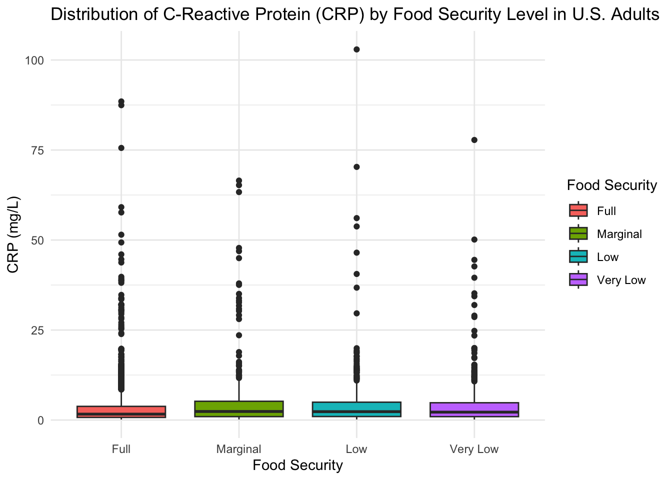
From this figure, we can see that there is considerable variability in CRP levels for all food security groups, as evidenced by the number of outliers appearing on the box plot. If we compare the median levels of CRP across the different food security groups, we see that the median CRP level for the “Full” food security group (CRP = 1.64) is slightly lower than the median CRP level for the “Marginal” (CRP = 2.38), “Low” (CRP = 2.33), and “Very Low” (CRP = 2.195) food security groups, which is in agreement with the results of Gowda et al. (2012).

In addition to looking at the raw values, levels of CRP can also be categorized based on risk for developing cardiovascular disease. The classifications for CRP are:

• Low (CRP < 1 mg/L)
• Moderate (1 mg/L \(\leq\) CRP \(\leq\) 3 mg/L)
• High (> 3 mg/L)

The figure below shows the percentage of subjects in each food security group that belong to each CRP risk class.

Code

sample <- sample %>%
  mutate(crp_group = case_when(
    crp_mgL < 1 ~ 'Low',
    crp_mgL >= 1 & crp_mgL <= 3 ~ 'Moderate',
    crp_mgL > 3 ~ 'High'
  ),
  crp_group = factor(crp_group, levels = c('Low', 'Moderate', 'High'))) 

sample %>%
  group_by(crp_group, hh_food_security) %>%
  summarize(count = n()) %>%
  left_join(counts_by_fs, by = 'hh_food_security') %>%
  mutate(percent = count/total) %>%
  ggplot(aes(x = hh_food_security, y = percent, fill = crp_group)) +
  geom_col(position='dodge') +
  theme_minimal() +
  scale_y_continuous(limits=c(0, 0.51), labels = scales::percent) +
  labs(
    title = 'CRP Risk Classification by Food Security Group',
    x = 'Food Security',
    y = 'Percent',
    fill = 'CRP Risk'
    )

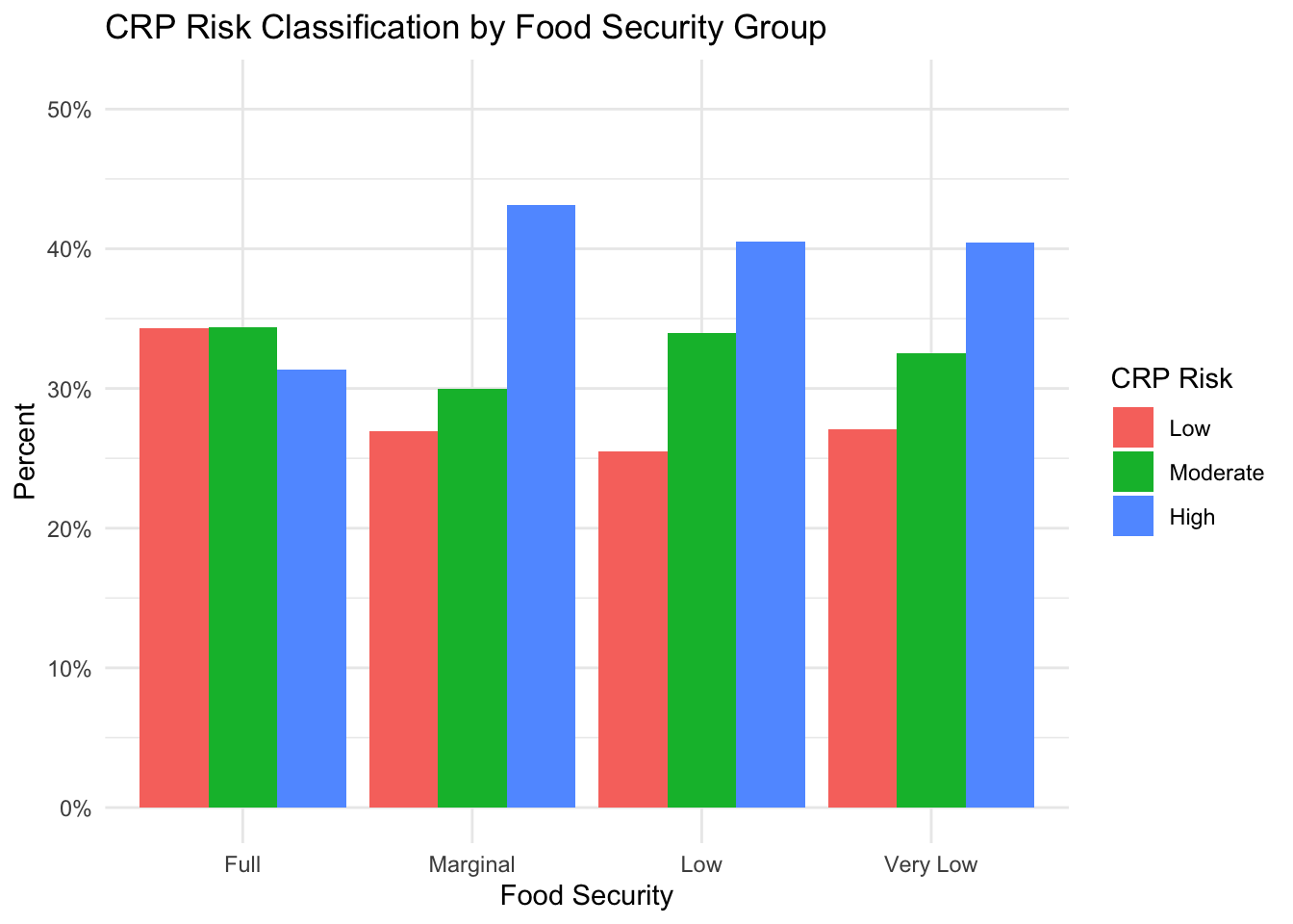
This figure shows that the group experiencing “Full” food security has a lower percentage of subjects in the high-risk CRP group (31%) than the “Marginal” (43%), “Low” (40%), and “Very Low” food security groups (40%). The “full” food security group also has a higher percentage of subjects in the low-risk CRP group (34%) than the groups experiencing reduced food security (“Marginal”: 27%, “Low”: 26%, “Very Low”: 27%). There does not, however, appear to be a clear relationship between food security level and the percentage of subjects with a moderate-risk CRP level.

Summary

Overall, the results of this analysis suggest that individuals experiencing food insecurity have higher levels of inflammation, as evidenced by higher levels of CRP in the blood stream, and a larger proportion of subjects in these groups have a level of CRP that is considered high-risk for future development of cardiovascular diseases.

RQ 2b: Can inflammation explain the observed health outcomes?

In RQ 1, we showed that the incidence of obesity, diabetes, and high blood pressure was higher in food-insecure groups. In RQ 2a, we showed elevated levels of CRP in groups experiencing reduced food security and an increased percentage of subjects with a CRP level that would be considered high-risk for downstream cardiovascular disease. Here, we aim to explore if elevated CRP levels could potentially explain the observed differences in incidence of metabolic conditions between the different food security groups.

Obesity

To begin, we will explore if the observed increase in incidence of obesity (as measured by BMI) in groups experiencing reduced food security can be explained by CRP levels.

The figure below shows the distribution of BMI classes by food security group and CRP risk class. To construct this figure, we start by dividing the data into 12 subgroups (one for each food security group and CRP risk level). Then, we plot the percentage of subjects within each subgroup that belong to each BMI class. As such, the bars in each grouped bar plot sum to 100%. To infer if CRP can explain the differences in obesity incidence, we can compare the BMI composition by CRP risk class for each food security group.

Code

sample <- sample %>%
  mutate(
    crp_group = case_when(
      crp_group == 'Low' ~ 'Low-Risk CRP',
      crp_group == 'Moderate' ~ 'Moderate-Risk CRP',
      crp_group == 'High' ~ 'High-Risk CRP'
      ),
      crp_group = factor(
        crp_group, 
        levels = c('Low-Risk CRP', 'Moderate-Risk CRP', 'High-Risk CRP')
        )
  ) 

# get counts for each food security and crp group
counts_by_fs <- sample %>%
    group_by(hh_food_security, crp_group) %>%
    summarize(total = n()) 

# plot
sample %>%
  group_by(bmi_class, hh_food_security, crp_group) %>%
  summarize(count = n()) %>%
  left_join(counts_by_fs, by = c('hh_food_security', 'crp_group')) %>%
  mutate(percent = count/total) %>%
  ggplot(aes(x = hh_food_security, y = percent, fill = bmi_class)) +
  geom_col(position='dodge') +
  facet_grid(vars(crp_group)) +
  theme_minimal() +
  scale_y_continuous(labels = scales::percent) +
  labs(
    title = 'BMI Distribution by Food Security Group and CRP Risk Class',
    x = 'Food Security',
    y = 'Percent',
    fill = 'BMI'
    )

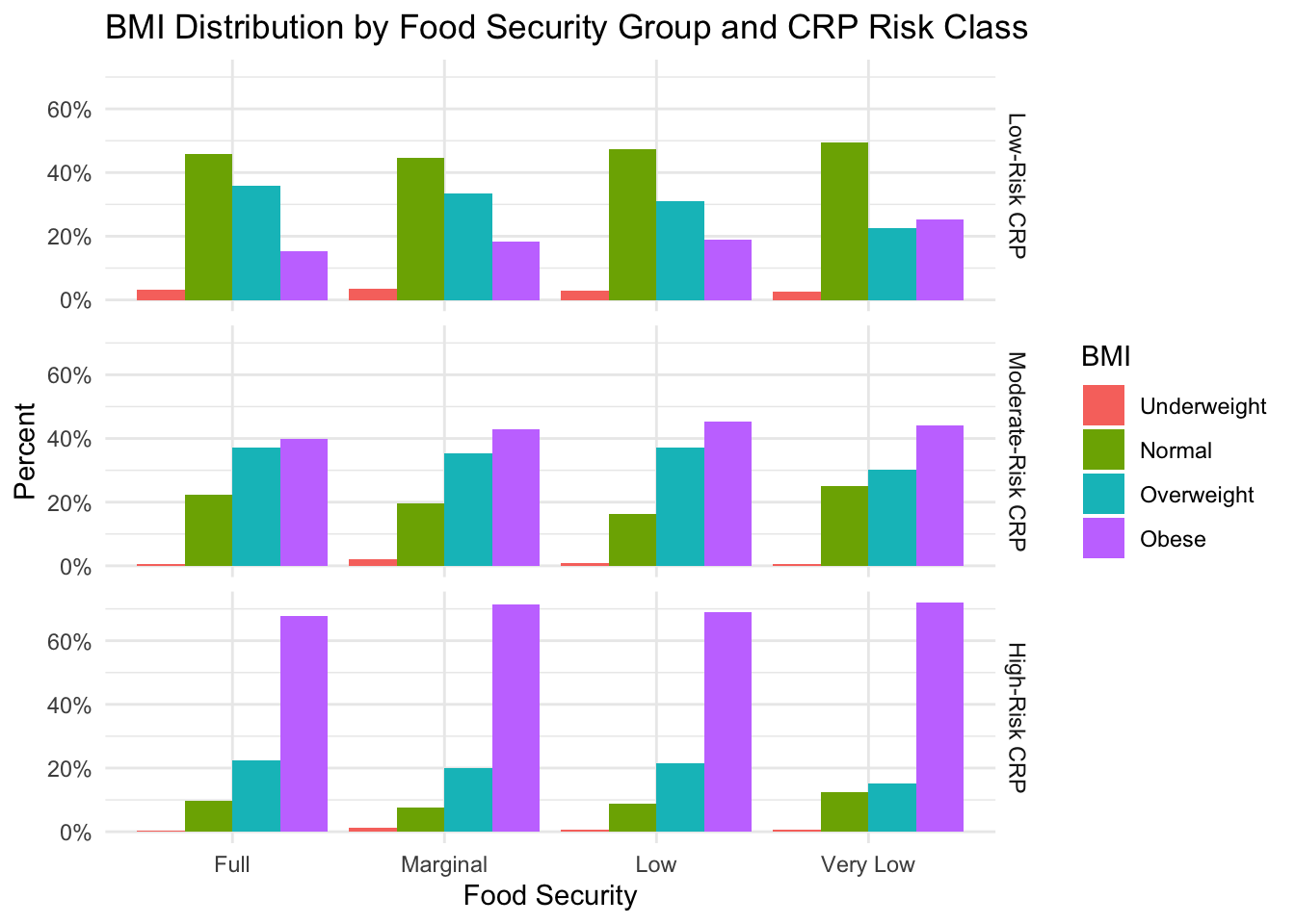
First, upon reviewing the graph, we can immediately see that the percentage of subjects with an obese BMI differs individually by CRP level and food security group. This is evidenced by 1) the “Full” food security group having a lower percentage of subjects with an obese BMI than the food-insecure groups, and 2) for all food security groups, the percentage of subjects with an obese BMI increases as CRP risk severity increases. Second, according to this figure, it does not appear that there is an interaction between CRP-risk severity and food security group. If we look down the column for each food security group, we see a similar trend in the percentage of BMI classes as CRP severity increases: the percentage of subjects with a normal BMI decreases and the percentage of subjects with an obese BMI increases.

Based on this analysis, it does not appear that CRP explains the differences in obesity incidence in our sample.

Diabetes

Next, we use a similar plot as above to explore if the increased incidence of diabetes in groups experiencing reduced food security could possibly be explained by CRP levels.

Code

sample %>%
  group_by(diabetes_all, hh_food_security, crp_group) %>%
  summarize(count = n()) %>%
  left_join(counts_by_fs, by = c('hh_food_security', 'crp_group')) %>%
  mutate(percent = count/total) %>%
  ggplot(aes(x = hh_food_security, y = percent, fill = diabetes_all)) +
  geom_col(position='dodge') +
  facet_grid(vars(crp_group)) +
  theme_minimal() +
  scale_y_continuous(labels = scales::percent) +
  labs(
    title = 'Diabetes Distribution by Food Security Group and CRP Risk Class',
    x = 'Food Security',
    y = 'Percent',
    fill = 'Diabetes'
    )

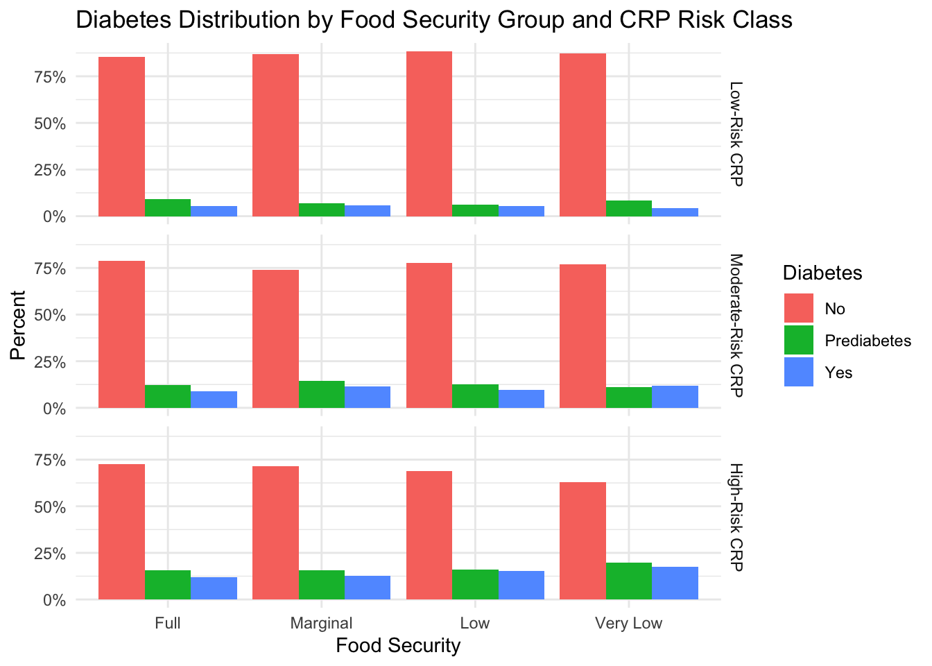
Again, when viewing this figure, we can immediately see individual effects of CRP level and food security group on diabetes status. This is evidenced by 1) unequal percentages of subjects with pre-diabetes and diabetes in the different food security groups, and 2) increasing incidence of prediabetes and diabetes with increasing CRP risk. Unlike obesity, however, there does appear to be an interaction between food security group and CRP risk severity. In the group of subjects with low-risk CRP levels, we see that the percentage of subjects with prediabetes or diabetes in the “Full” food security group (15%) is slightly higher than the percentage of subjects with prediabetes or diabetes in the “Marginal” (13%), “Low” (11%), or “Very Low” (12%) food security groups. As the risk associated with the CRP level increases, however, the trend switches. At moderate CRP risk, we see that the percentage of subjects with prediabetes or diabetes in the “Full” food security group (21%) is slightly lower than the percentage of subjects with prediabetes or diabetes in the “Marginal” (26%), “Low” (23%), or “Very Low” (23%) food security groups. This trend continues at the highest CRP risk level (“Full”: 28%, “Marginal”: 29% , “Low”: 31%, “Very Low”: 37%).

Because diabetes incidence is lower in food-secure groups when CRP levels are lower, these results could suggest that diabetes prevalence in groups experiencing food insecurity is more highly dependent on CRP levels than in groups experiencing food security.

High Blood Pressure

Finally, we perform a final analysis to explore if the increased incidence of high blood pressure in groups experiencing reduced food security could possibly be explained by CRP levels.

Code

sample %>%
  group_by(high_bp, hh_food_security, crp_group) %>%
  summarize(count = n()) %>%
  left_join(counts_by_fs, by = c('hh_food_security', 'crp_group')) %>%
  mutate(percent = count/total) %>%
  ggplot(aes(x = hh_food_security, y = percent, fill = high_bp)) +
  geom_col(position='dodge') +
  facet_grid(rows = vars(crp_group)) +
  theme_minimal() +
  scale_y_continuous(labels = scales::percent) +
  labs(
    title = 'Blood Pressure Classification by Food Security Group and CRP Level',
    x = 'Food Security',
    y = 'Percent',
    fill = 'High Blood Pressure'
    )

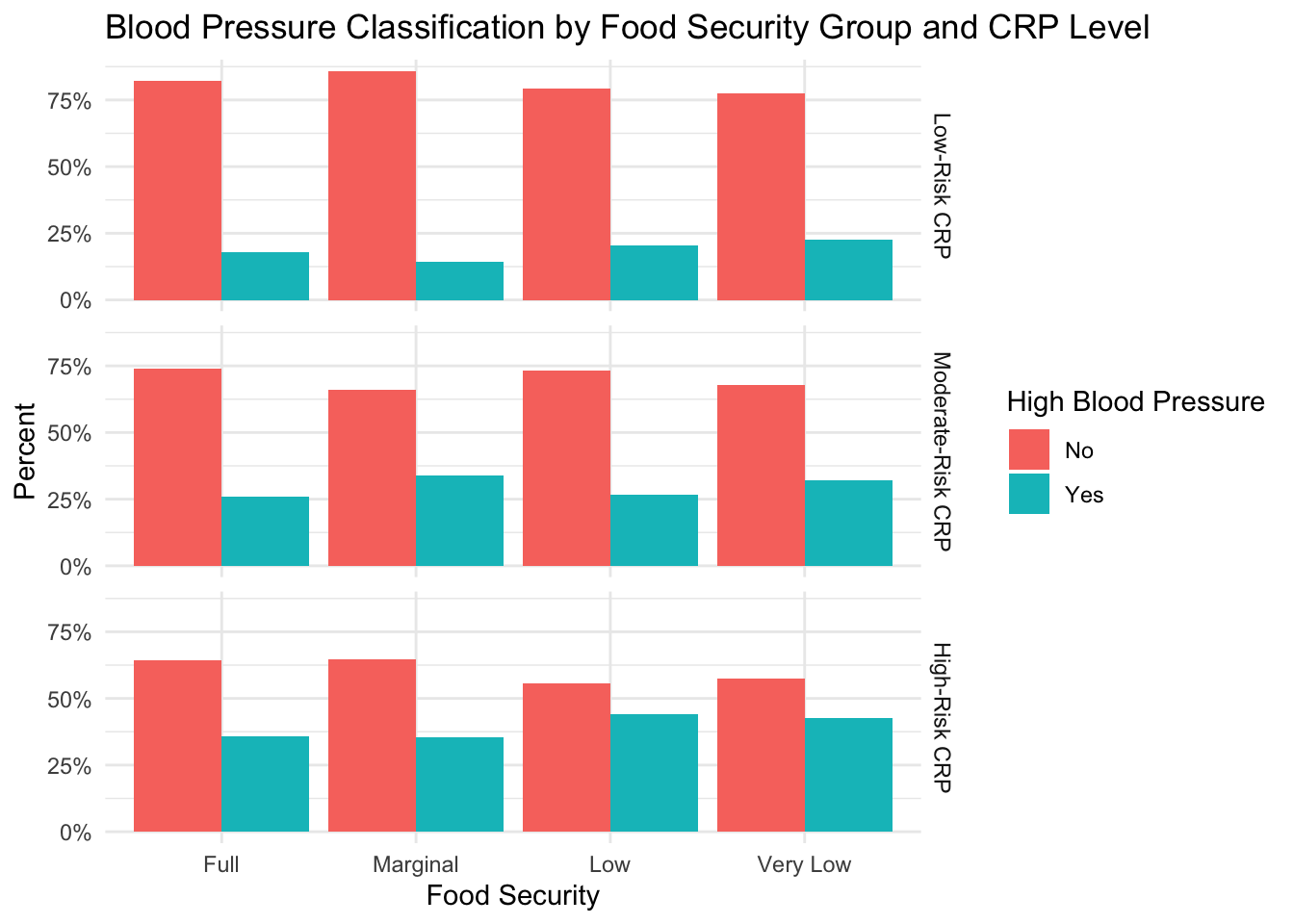
From this figure, we can see the individual effects of food security group and CRP level on incidence of high blood pressure. There are unequal percentages of subjects with high blood pressure in the different food security groups, and there is an increased incidence of high blood pressure as the CRP risk increases. Similar to diabetes, however, there does appear to be a slight interaction between CRP risk and food security group. Specifically, in the figure, we can see that at the lowest level of CRP risk, the “Marginal” food security group has the lowest percentage of subjects with high blood pressure. At moderate CRP risk, the “Full” and “Very Low” food security groups have the lowest percentage of subjects with high blood pressure, while the “Marginal” food security group has the highest. In the group of subjects with high-risk CRP levels, we see that the “Low” and “Very Low” food security groups have the highest proportion of subjects with high blood pressure. The results of these analyses could suggest a more severe impact of high CRP on the development of high blood pressure in the “Low” and “Very Low” food security groups, but more research would be warranted.

Conclusion

Overall, for this project, we explored the impact of food security level on health outcomes and inflammation in U.S. adults. Our findings suggest increased incidence of obesity, diabetes, and high blood pressure in adults experiencing reduced food security, and levels of high-risk CRP are more prevalent in this group. Additionally, we showed an interaction effect between food security group and CRP level for diabetes and high blood pressure, which suggests that CRP levels could potentially explain the increased incidence of these conditions in food-insecure individuals. However, to quantify these relationships–and control for potential confounding factors–statistical analyses should be conducted.

Limitations

There are several limitations to our exploratory analyses of this data.

• Metabolic Outcome Variables. For several of the metabolic conditions, including diabetes, high cholesterol, and high blood pressure, we were limited to self-reported “Yes”/“No” variables to indicate if a subject had previously been diagnosed with the disorder. This type of variable can be unreliable as it requires a patient to have a diagnosis and be honest about the result. Additionally, given that health-seeking behaviors can vary by individual, it is possible that some subjects have a higher likelihood of knowing their disease status than others. A better outcome variable would have been to obtain a quantitative lab value to assess these conditions. However, given that patients often take medications to control for diabetes, cholesterol, and blood pressure, it is also unlikely that these values would have reflected diagnosis of one of the health conditions. If I were to repeat this analysis, I would likely engineer a variable for each condition that accounts for self-reported diagnosis, medication to control the disorder, and lab values to indicate undiagnosed disease.

• Confounding Factors. When describing our sample, we found differences in several demographic and lifestyle factors that could potentially influence both health outcomes and inflammatory status, such as age, smoking, and socioeconomic factors. To prevent figures from becoming too complicated, I chose to omit the influence of any compounding factors from analyses. However, in order to truly parse out how much variation can be explained by food security group, any future statistical analyses should control for confounding variables.

• Inequality of food security group sizes. As found in the U.S. population, our study sample exhibits a class imbalance between people who are fully food-secure and the groups experiencing some form of food insecurity. To increase confidence in our findings, we might wish to increase the number of food insecure individuals in our sample. Additionally, the unequal sample sizes meant that percentages were used for all of comparisons. Percentages can vary greatly by sample size, which is another limitation of this project.

• Visualizing mediation effects. To see if CRP levels could explain the relationship between health outcomes and food security group, bar plots faceted by CRP level were used. It is possible that this was not the right approach to study this relationship. A more thorough approach would be to conduct a statistical analysis, where CRP level can be a mediator.

• Psychological impact of food insecurity. One limitation of this dataset is that it does not allow us to quantify the difficulty that food insecurity imposes on individual subjects’ lives. Because stress is known to exacerbate many health outcomes, it would be interesting to understand how the psychological distress associated with food insecurity impacts inflammation.

References

• Berkowitz, S.A., Baggett, T.P., Wexler, D.J., Huskey, K.W., & Wee, C.C. (2013). Food insecurity and metabolic control among U.S. adults with diabetes. Diabetes Care, 36, 3093–9.

• Bermudez-Millan, A., Wagner, J.A., Feinn, R.S., Segura-Perez, S., Damio, G., Chhabra, J., & Perez-Escamilla, R. (2019). Inflammation and Stress Biomarkers Mediate the Association between Household Food Insecurity and Insulin Resistance among Latinos with Type 2 Diabetes, Journal of Nutrition, 982-988.

• Broussard, N.H. (2019). What explains gender differences in food insecurity?, Food Policy, 83, 180-194.

• Burgess, L. (2017). Why is the hip-waist ratio important?. MedicalNewsToday. Link

• Gowda, C., Hadley, C., & Aiello, A.E. (2012). The Association Between Food Insecurity and Inflammation in the US Adult Population. American Journal of Public Health, 102(8), 1579-1586.

• Grolemund, G., & Wickham, H. (2017). R for Data Science. O’Reilly Media.

• Harvard Health Publishing. (2017). C-Reactive Protein test to screen for heart disease: Why do we need another test? Link

• Hernandez, D.C., Reesor, L.M, & Murillo R. (2017). Food insecurity and adult overweight/obesity: gender and race/ethnic disparities. Appetite 117, 373–8.

• Kroenke, K., Spitzer, R. L., & Williams, J. B. (2001). The PHQ-9: validity of a brief depression severity measure. Journal of General Internal Medicine, 16(9), 606-613

• National Center for Health Statistics (2020). National Health and Nutrition Examination Survey Data. U.S. Department of Health and Human Services, Centers for Disease Control and Prevention.

• R Core Team. (2023). R: A Language and Environment for Statistical Computing. R Foundation for Statistical Computing. https://www.R-project.org/

• United States Department of Agriculture, Economic Research Service. (2023). Key statistics & graphics. Link

• Zierath, R., Clagget, B., Hall, M.E., Correa, A., Barber, S., Gao, Y., Talegawkar, S., Ezekwe, E.I., Tucker, K., Diez-Rouz, A.V., Sims, M. & Shah, A.M. (2023). Measures of Food Inadequacy and Cardiovascular Disease Risk in Black Individuals in the US From the Jackson Heart Study. JAMA Network Open.