Code
library(tidyverse)
library(here)
library(glue)
library(haven)
library(purrr)
library(ggplot2)
knitr::opts_chunk$set(echo = TRUE)library(tidyverse)
library(here)
library(glue)
library(haven)
library(purrr)
library(ggplot2)
knitr::opts_chunk$set(echo = TRUE)The United States Department of Agriculture (USDA) defines household food security as having enough food so that all members of a household can live an active, healthy life (USDA, 2023). Conversely, food insecurity is characterized by being unable to attain enough food to meet the needs of all members of a household. In 2021, it was estimated that approximately 10.2% of households in the United States (13.5 million households) experienced some form of food insecurity in 2021.
Given the important role that food and nutrition play in health outcomes, research has been conducted to understand the relationship between food insecurity and metabolic health outcomes. Results have shown a significant relationship between food insecurity and several conditions, such as obesity (Hernandez, Reesor, & Murillo, 2017), insulin resistance (Bermudez-Millan et al., 2019), diabetes (Berkowitz et al., 2013), and cardiovascular diseases (Zierath et al., 2023).
C-reactive protein (CRP) is an inflammatory biomarker that is produced by the liver. Traditionally, it has been found to be elevated during instances of inflammation or infection. However, medical research has highlighted its ability to detect inflammation in blood vessels, and elevated CRP is now a leading predictor for cardiovascular diseases (Harvard Health Publishing, 2017).
Given the association between food insecurity and increased incidence of metabolic conditions and heart disease, research has also focused on understanding the role that inflammatory biomarkers, such as CRP, could play in the onset of these conditions. Indeed, Gowda et al. (2012) found higher levels of CRP in U.S. adults experiencing food insecurity.
The goal of this project will be to replicate and expand upon the work of Gowda et al. (2012) by conducting an exploration of food security status, health outcomes, and inflammation in U.S. adults.
This analysis utilizes data from the National Health and Nutrition Examination Survey (NHANES), an annual survey conducted by the National Center for Health Statistics (NCHS) that assesses the health and nutritional status of adults and children. Data is collected through comprehensive interviews and physical and laboratory examinations and is released on a biennial basis. Each year, approximately 5,000 Americans are chosen for inclusion in the survey, and the population sampled is designed to be representative of the United States population.
NHANES data is divided into five main categories:
Demographics Data: Demographic and socioeconomic information about study participants, such as country of birth, education level, gender, race, and age.
Dietary Data: Information about supplement-use and food/nutritional intake
Examination Data: Information that comes from a physical examination, such as blood pressure, anthropomorphic measures (e.g. weight), and oral health.
Laboratory Data: Information that comes from serum lab tests, such as blood lipids, liver proteins, and many others.
Questionnaire Data: Information that comes from an interview, including personal and family health history, medication use, physical activity, and many others.
Across these five categories, the full NHANES dataset includes approximately 94 tables, but we will only use 12 tables (or possibly fewer) for our analysis. All of the tables can be easily joined using the subject’s unique identification number.
The website for NHANES currently has data dating back to 1999 available to the public, but for this analysis, we will focus on the data collected from January 2017 to March 2020 (pre-pandemic data).
base_path <- here('posts', '_data', 'nhanes')
read_data_from_base <- function(path) {
return(read_xpt(glue('{base_path}/{path}')))
}
# Questionnaire data
demo <- read_data_from_base('P_DEMO.XPT')
bp_chol <- read_data_from_base('P_BPQ.XPT')
depression <- read_data_from_base('P_DPQ.XPT')
diabetes <- read_data_from_base('P_DIQ.XPT')
exercise <- read_data_from_base('P_PAQ.XPT')
food_security <- read_data_from_base('P_FSQ.XPT')
# health_conditions <- read_data_from_base('P_MCQ.XPT')
insurance <- read_data_from_base('P_HIQ.XPT')
nutrition <- read_data_from_base('P_DBQ.XPT')
# Physical exam data
body <- read_data_from_base('P_BMX.XPT')
# Labs data
bc_count <- read_data_from_base('P_CBC.XPT')
cotinine <- read_data_from_base('P_COT.XPT')
crp <- read_data_from_base('P_HSCRP.XPT')In order to use this data for exploratory data analysis, we must first clean the data. For each data table, we will:
mutate to create new columns that can be used in our analysisA cleaned version of the data is shown for each table.
select_relevant_cols <- function(df, cols_list) {
df <- df %>%
select(all_of(cols_list))
return(df)
}The Demographics dataset provides demographic information for all study participants (n = 15560). The raw dataset contains 29 columns, but we will limit the data to only include the identifier column, age, gender, race/ethnicity, and income to poverty ratio.
demo_cols <- c('SEQN', 'RIAGENDR', 'RIDAGEYR', 'RIDRETH3', 'INDFMPIR')
demo_clean <- demo %>%
select_relevant_cols(demo_cols) %>%
rename(
id = SEQN,
gender = RIAGENDR,
age = RIDAGEYR,
race = RIDRETH3,
income_poverty_ratio = INDFMPIR
) %>%
mutate(
gender = case_when(
gender == 1 ~ 'M',
gender == 2 ~ 'F',
gender == '.' ~ NA
),
gender = factor(gender, levels = c('M', 'F')),
race = case_when(
race == 1 ~ 'Mexican American',
race == 2 ~ 'Other Hispanic',
race == 3 ~ 'Non-Hispanic White',
race == 4 ~ 'Non-Hispanic Black',
race == 6 ~ 'Non-Hispanic Asian',
race == 7 ~ 'Other Race',
race == '.' ~ NA
),
race = factor(race)
)
demo_cleanBlood Pressure and Cholesterol
The Blood Pressure and Cholesterol dataset contains information about each subject’s blood pressure and cholesterol status. The raw dataset contains data for a subset of NHANES participants (n = 10195) and consists of 11 columns. For our analyses, we will only use the columns that indicate if a subject has been told that they have high blood pressure or high cholesterol.
bp_chol_cols <- c('SEQN', 'BPQ020', 'BPQ080')
bp_chol_clean <- bp_chol %>%
select_relevant_cols(bp_chol_cols) %>%
rename(
id = SEQN,
high_bp = BPQ020,
high_cholesterol = BPQ080
) %>%
mutate(
across(
c(high_bp, high_cholesterol),
~case_when(.x == 1 ~ 'Yes',
.x == 2 ~ 'No',
.x %in% c(7, 9) ~ NA,
.x == '.' ~ NA)
),
high_bp = factor(high_bp, levels = c('Yes', 'No')),
high_cholesterol = factor(high_cholesterol, levels = c('Yes', 'No'))
)
bp_chol_cleanDiabetes
The Diabetes dataset contains information about each subject’s diabetes status. The raw dataset contains data for a subset of NHANES participants (n = 14986) and consists of 28 columns. For our analyses, we will only use the columns that indicate if a subject has been told that they have diabetes or pre-diabetes.
diabetes_cols <- c('SEQN', 'DIQ010', 'DIQ160')
diabetes_clean <- diabetes %>%
select_relevant_cols(diabetes_cols) %>%
rename(
id = SEQN,
diabetes = DIQ010,
pre_diabetes = DIQ160
) %>%
mutate(
diabetes = case_when(
diabetes == 1 ~ 'Yes',
diabetes == 2 ~ 'No',
diabetes == 3 ~ 'Borderline',
diabetes %in% c(7, 9) ~ NA,
diabetes == '.' ~ NA
),
diabetes = factor(diabetes, levels = c('No', 'Borderline', 'Yes')),
pre_diabetes = case_when(
pre_diabetes == 1 ~ 'Yes',
pre_diabetes == 2 ~ 'No',
pre_diabetes %in% c(7, 9) ~ NA,
pre_diabetes == '.' ~ NA
),
pre_diabetes = factor(pre_diabetes, levels = c('No', 'Yes'))
)
diabetes_cleanDiet Behavior and Nutrition
The Diet Behavior and Nutrition dataset provides information about a subject’s dietary habits and a self-evaluation of the healthiness of their diet. The raw dataset contains data for all NHANES participants (n = 15560) and consists of 46 columns. For our analyses, we will only use the columns that describe the healthiness of the diet and dietary patterns in terms of types of meals that are consumed (e.g. frozen food, fast food, read-to-eat meals etc).
nutrition_cols <- c('SEQN', 'DBQ700', 'DBD895', 'DBD900', 'DBD905', 'DBD910')
nutrition_clean <- nutrition %>%
select_relevant_cols(nutrition_cols) %>%
rename(
id = SEQN,
health_diet = DBQ700,
n_meals_out = DBD895,
n_meals_ff = DBD900,
n_rte_meals = DBD905,
n_frozen_meals = DBD910
) %>%
mutate(
health_diet = case_when(
health_diet == 1 ~ 'Excellent',
health_diet == 2 ~ 'Very good',
health_diet == 3 ~ 'Good',
health_diet == 4 ~ 'Fair',
health_diet == 5 ~ 'Poor',
health_diet %in% c(7, 9) ~ NA,
health_diet == '.' ~ NA
),
health_diet = factor(health_diet, levels = c('Poor', 'Fair', 'Good', 'Very good', 'Excellent')),
across(c('n_meals_out', 'n_meals_ff', 'n_rte_meals', 'n_frozen_meals'), ~ifelse((.x %in% c(5555, 7777, 9999)) | (.x == '.'), NA, .x))
)
nutrition_cleanExercise
The Physical Activity dataset contains data to describe the amount of physical activity that a subject gets on a daily and weekly basis. The raw dataset contains data for a subset of NHANES participants (n = 9693) and consists of 17 columns. Although the dataset contains information about physical activity performed through work, transportation, and recreation, for our analyses, we will only use the columns that describe a subject’s sedentary activity and recreational physical activity.
exercise_cols <- c('SEQN', 'PAQ650', 'PAQ665', 'PAD680')
exercise_clean <- exercise %>%
select_relevant_cols(exercise_cols) %>%
rename(
id = SEQN,
vigorous_exercise = PAQ650,
moderate_exercise = PAQ665,
sedentary_minutes = PAD680
) %>%
mutate(
across(
c(vigorous_exercise, moderate_exercise),
~case_when(.x == 1 ~ 'Yes', .x == 2 ~ 'No', .x %in% c(7, 9) ~ NA, .x == '.' ~ NA)
),
vigorous_exercise = factor(vigorous_exercise, levels = c('Yes', 'No')),
moderate_exercise = factor(moderate_exercise, levels = c('Yes', 'No')),
sedentary_minutes = ifelse((sedentary_minutes %in% c(7777, 9999)) | (sedentary_minutes == '.'), NA, sedentary_minutes)
)
exercise_cleanFood Security
The Food Security dataset contains information about individual and household access to food and food-related benefits. The raw dataset contains data for all NHANES participants (n = 15560) and consists of 20 columns. For our analysis, we will explore household food security and household access to food benefits (e.g. SNAP, food stamps) and emergency food (e.g. food banks, soup kitchens) in the last 12 months.
food_security_cols <- c('SEQN', 'FSDHH', 'FSD151', 'FSQ012')
food_security_clean <- food_security %>%
select_relevant_cols(food_security_cols) %>%
rename(
id = SEQN,
hh_food_security = FSDHH,
hh_emergency_food = FSD151,
hh_fs_benefit = FSQ012
) %>%
mutate(
hh_food_security = case_when(
hh_food_security == 1 ~ 'Full',
hh_food_security == 2 ~ 'Marginal',
hh_food_security == 3 ~ 'Low',
hh_food_security == 4 ~ 'Very Low',
hh_food_security == '.' ~ NA
),
hh_food_security = factor(hh_food_security, levels = c('Full', 'Marginal', 'Low', 'Very Low')),
across(c(hh_emergency_food, hh_fs_benefit),
~case_when(.x == 1 ~ T,
.x == 2 ~ F,
.x %in% c(7, 9) ~ NA,
.x == '.' ~ NA))
)
food_security_cleanMental Health Screener
To screen participants’ mental health, NHANES administers the Patient Health Questionnaire (PHQ). The PHQ contains 9 questions that assess the frequency of depressive symptoms over a two week period. For each question, the participant can indicate if they’ve experienced the symptom “Not at all”, “Several Days”, “More than half the days”, or “Nearly every day”, and points ranging from 0 to 3 are assigned according to the response. The scores on each question are summed to produce a final score that ranges from 0 to 27.
This dataset contains PHQ data for a subset of NHANES subjects (n = 8965) participants. For this analysis, we will only use the final score.
q_cols <- colnames(depression %>% select(-DPQ100, -SEQN))
depression_clean <- depression %>%
mutate(across(everything(), ~ifelse(. %in% c(7, 9), NA, .))) %>%
mutate(across(everything(), ~ifelse(. == '.', NA, .))) %>%
rowwise() %>%
mutate(total_score = sum(across(all_of(q_cols)))) %>% # do not remove NA!
ungroup() %>%
select(id = SEQN, total_score, -all_of(q_cols))
depression_cleanInsurance
The Health Insurance dataset contains information about individual health insurance coverage. The raw dataset contains data for all NHANES participants (n = 15560) and consists of 14 columns, including data for many types of health insurance (e.g. private, Medicare, Medicaid). For our analysis, we will limit our data to the column that indicates if a subject is covered by any type of health insurance.
insurance_cols <- c('SEQN', 'HIQ011')
insurance_clean <- insurance %>%
select_relevant_cols(insurance_cols) %>%
rename(
id = SEQN,
has_med_insurance = HIQ011
) %>%
mutate(
has_med_insurance = case_when(
has_med_insurance == 1 ~ 'Yes',
has_med_insurance == 2 ~ 'No',
has_med_insurance %in% c(7, 9) ~ NA,
has_med_insurance == '.' ~ NA),
has_med_insurance = factor(has_med_insurance, levels = c('No', 'Yes'))
)
insurance_cleanBody Measures
The Body Measures dataset provides information about a subject’s build. The raw dataset contains data for all NHANES participants (n = 14300) and consists of 22 columns. For our analysis, we will utilize the variables related to BMI, and waist and hip circumference. Because the waist-to-hip ratio can be an indicator of abdominal obesity, we will also engineer this feature (in case we want to use it later on).
body_cols <- c('SEQN', 'BMXBMI', 'BMXWAIST', 'BMXHIP')
body_clean <- body %>%
select_relevant_cols(body_cols) %>%
mutate(across(body_cols[body_cols != 'SEQN'], ~ifelse(.x == '.', NA, .x))) %>%
rename(
id = SEQN,
bmi = BMXBMI,
waist_circ = BMXWAIST,
hip_circ = BMXHIP
) %>%
mutate(waist_hip_ratio = round(waist_circ/hip_circ, 2))
body_cleanBlood Cell Count
The Complete Blood Count dataset provides a count of blood cells, including red blood cells, white blood cells, and platelets, as well as other details. The raw dataset contains data for a subset of NHANES participants (n = 13772) and consists of 22 columns. For our analysis, we will only be interested in White Blood Cells counts, and we will engineer a feature to indicate if a subject has elevated white blood cells (cell count > 11,000 cells/microliter). Elevated white blood cells could be indicative of infection or a more serious health condition and could impact analyses of other lab variables, such as CRP (below).
bc_count_cols <- c('SEQN', 'LBXWBCSI')
bc_count_clean <- bc_count %>%
select_relevant_cols(bc_count_cols) %>%
rename(id = SEQN, wbc = LBXWBCSI) %>%
mutate(elevated_wbc = ifelse(wbc > 11, T, F))
bc_count_cleanCotinine
Cotinine is a metabolite of nicotine, and its presence in blood can be used to measure an individual’s exposure to tobacco smoke or tobacco use. For this analysis, we use the Cotinine dataset to engineer features related to tobacco exposure and smoking status. We first use the criteria presented in Gowda, Hadley, & Aiello (2012) to classify tobacco exposure levels based on serum cotinine level. Next, we use the exposure classifications to classify a subject as a smoker or non-smoker.
The raw dataset contains data for a subset of NHANES subjects (n = 13027).
cotinine_cols <- c('SEQN', 'LBXCOT', 'LBDCOTLC')
cotinine_clean <- cotinine %>%
select_relevant_cols(cotinine_cols) %>%
rename(
id = SEQN,
cot = LBXCOT,
quality = LBDCOTLC
) %>%
# if not detectable, count as 0 exposure
mutate(
cot = ifelse(quality == 1, 0, cot)
) %>%
select(-quality) %>%
mutate(
tob_exp_level = case_when(
cot == 0 ~ 'None',
cot <= 15 ~ 'Secondhand',
cot > 15 ~ 'Smoker',
T ~ NA
),
tob_exp_level = factor(tob_exp_level, levels = c('None', 'Secondhand', 'Smoker')),
smoker = case_when(
tob_exp_level %in% c('None', 'Secondhand') ~ 'Non-Smoker',
tob_exp_level == 'Smoker' ~ 'Smoker',
T ~ NA
),
smoker = factor(smoker, levels = c('Non-Smoker', 'Smoker'))
)
cotinine_cleanC-Reactive Protein
The high-sensitivity CRP dataset provides serum levels for C-Reactive Protein, an inflammatory biomarker. The raw dataset contains CRP measures for all NHANES participants (n = 13772). There are three columns, corresponding to the participant ID, CRP measure (mg/L), and a quality metric. We will set any readings below the detection limit to NA.
crp_cols <- c('SEQN', 'LBXHSCRP', 'LBDHRPLC')
crp_clean <- crp %>%
select_relevant_cols(crp_cols) %>%
rename(
id = SEQN,
crp_mgL = LBXHSCRP,
quality = LBDHRPLC
) %>%
# if not at detection limit, set crp to NA
mutate(crp_mgL = ifelse(quality == 0, crp_mgL, NA)) %>%
select(-quality)
crp_cleanFinally, now that we have cleaned each individual dataset, we can use a left_join to combine our 12 datasets into a single dataset.
df_to_join <- list(
demo_clean,
bp_chol_clean,
depression_clean,
diabetes_clean,
exercise_clean,
food_security_clean,
insurance_clean,
nutrition_clean,
body_clean,
bc_count_clean,
cotinine_clean,
crp_clean
)
# use purrr to join all data frames with one function call!
# https://stackoverflow.com/questions/32066402/how-to-perform-multiple-left-joins-using-dplyr-in-r
full_df <- reduce(df_to_join, left_join, by = 'id')
full_dfThe joined data contains data for 15560 subjects.
We will require that all NHANES subjects be 18-64 years of age for inclusion in our analysis. We will exclude any subjects with a white blood cell count that is greater than 11,000 cells/ microliter of blood (as this could indicate an infection or more serious health condition, such as cancer). Additionally, we will exclude any subjects missing data in the columns needed for our primary analysis: gender, age, race, income-to-poverty ratio, medical insurance coverage, health outcomes (high_bp, high_cholesterol, diabetes, bmi), household food security, smoker status, and C-reactive protein.
core_cols <- c('gender', 'age', 'race', 'income_poverty_ratio', 'high_bp', 'high_cholesterol', 'diabetes', 'hh_food_security', 'bmi', 'waist_hip_ratio', 'has_med_insurance', 'smoker', 'crp_mgL')
sample <- full_df %>%
filter(
age > 18,
age < 64,
elevated_wbc != T) %>%
# https://stackoverflow.com/questions/33520854/filtering-data-frame-based-on-na-on-multiple-columns
filter_at(vars(core_cols), all_vars(!is.na(.)))
sampleThis leaves us with a sample of size of 4584 subjects.
Because we are interested in exploring health outcomes by food security status, we will begin by understanding the distribution of food security levels in our sample and any demographic or lifestyle changes that are immediately observed between these groups.
Distribution of Food Security Levels
sample %>%
ggplot(aes(x=hh_food_security)) +
geom_bar() +
theme_minimal() +
labs(
title = 'Household Food Security in our sample of U.S. Adults',
x = 'Food Security Classification',
y = 'Count'
)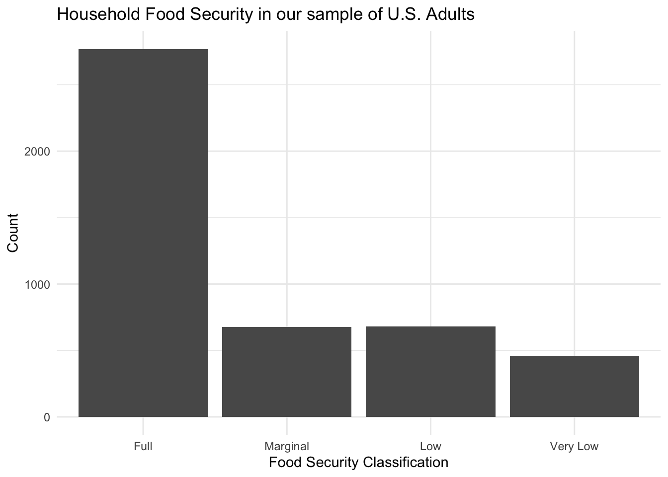
From this figure, we can see that the majority of subjects in our sample are fully food secure. Approximately 1/3 of our sample, however, has experienced some level of food insecurity.
Distribution of Age by Food Security Levels
sample %>%
ggplot(aes(x=age, colour = hh_food_security)) +
geom_density() +
# facet_grid(rows = vars(hh_food_security)) +
theme_minimal() +
labs(
title = 'Age Distribution by Household Food Security in our sample of U.S. Adults',
x = 'Age',
y = 'Density'
)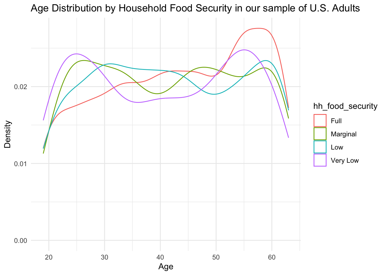
From the above density plot, we see that there is a peak at the ages 50-60 for fully food-secure subjects, indicating that older individuals might be more food secure. Additionally, we see an interesting bimodal distribution within the very low food security group. It appears that there is a peak of individuals experiencing food insecurity at both the younger ages (20-30) and older ages (50-55).
Distribution of Gender by Food Security Levels
counts_by_fs <- sample %>%
group_by(hh_food_security) %>%
summarize(total = n())
sample %>%
group_by(gender, hh_food_security) %>%
summarize(count = n()) %>%
left_join(counts_by_fs, by = 'hh_food_security') %>%
mutate(percent = count/total) %>%
ggplot(aes(x = hh_food_security, y = percent, fill = gender)) +
geom_col(position = 'dodge') +
# facet_grid(rows = vars(hh_food_security)) +
theme_minimal() +
scale_y_continuous(labels = scales::percent) +
labs(
title = 'Gender Distribution by Household Food Security in our sample of U.S. Adults',
x = 'Food Security Classification',
y = 'Percent',
fill = 'Gender'
)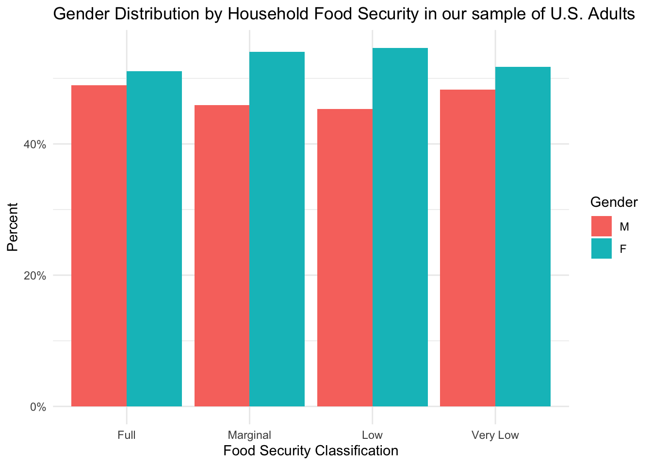
This figure shows that each group has more females than males, but this difference is more pronounced in groups experiencing food insecurity.
Distribution of Smoking Status by Food Security Levels
counts_by_fs <- sample %>%
group_by(hh_food_security) %>%
summarize(total = n())
sample %>%
group_by(smoker, hh_food_security) %>%
summarize(count = n()) %>%
left_join(counts_by_fs, by = 'hh_food_security') %>%
mutate(percent = count/total) %>%
ggplot(aes(x = hh_food_security, y = percent, fill = smoker)) +
geom_col(position = 'dodge') +
# facet_grid(rows = vars(hh_food_security)) +
theme_minimal() +
scale_y_continuous(labels = scales::percent) +
labs(
title = 'Smoker Distribution by Household Food Security in our sample of U.S. Adults',
x = 'Food Security Classification',
y = 'Percent',
fill = 'Gender'
)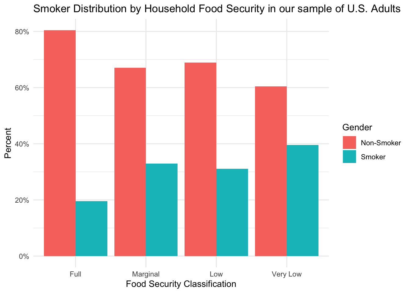
From this figure, we can see that the full food-security group appears to contain a higher percentage of non-smokers than any of the other groups. When interpreting differences in health outcomes, this could be an important factor to consider.
Distribution of Income-Poverty Ratio by Food Security Levels
sample %>%
ggplot(aes(x=income_poverty_ratio, colour = hh_food_security)) +
geom_density() +
# facet_grid(rows = vars(hh_food_security)) +
theme_minimal() +
labs(
title = 'Distribution of Income-Poverty Ratio by Household Food Security in our sample of U.S. Adults',
x = 'Income-Poverty Ratio',
y = 'Density'
)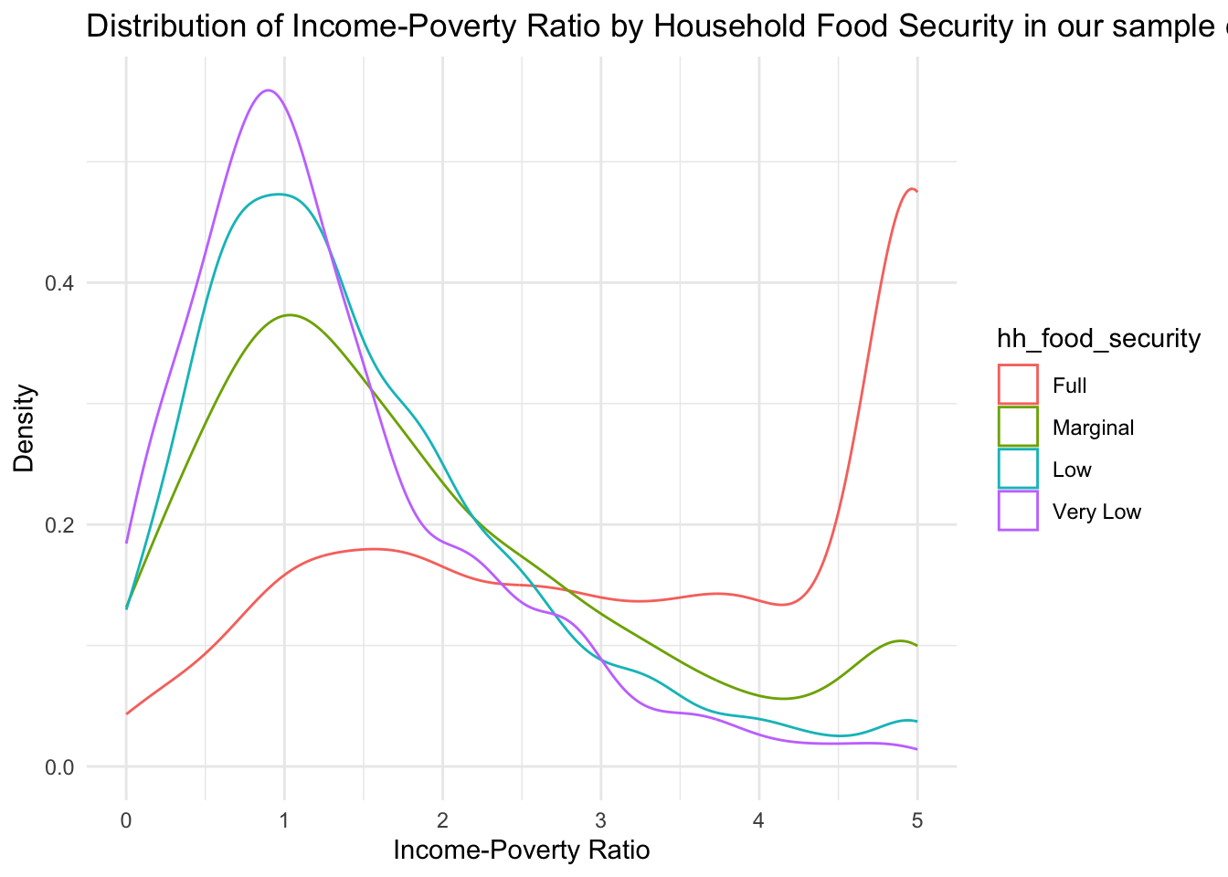
From this table, we can see that a higher proportion of subjects in the full food security group has a very high income-to-poverty ratio, indicating a salary that is ~5x as high as the federal poverty cut-off. Oppositely, the groups indicating some degree of food insecurity have a large proportion of subjects with low income-poverty ratios. For the very low food secure group, the peak is located to the left of the 1 marker, indicating a large proportion of subjects living below the poverty line.
Distribution of Health Insurance Coverage by Food Security Levels
counts_by_fs <- sample %>%
group_by(hh_food_security) %>%
summarize(total = n())
sample %>%
group_by(has_med_insurance, hh_food_security) %>%
summarize(count = n()) %>%
left_join(counts_by_fs, by = 'hh_food_security') %>%
mutate(percent = count/total) %>%
ggplot(aes(x = hh_food_security, y = percent, fill = has_med_insurance)) +
geom_col(position = 'dodge') +
# facet_grid(rows = vars(hh_food_security)) +
theme_minimal() +
scale_y_continuous(labels = scales::percent) +
labs(
title = 'Distribution of Medical Coverage by Household Food Security in our sample of U.S. Adults',
x = 'Food Security Classification',
y = 'Percent',
fill = 'Medical Coverage'
)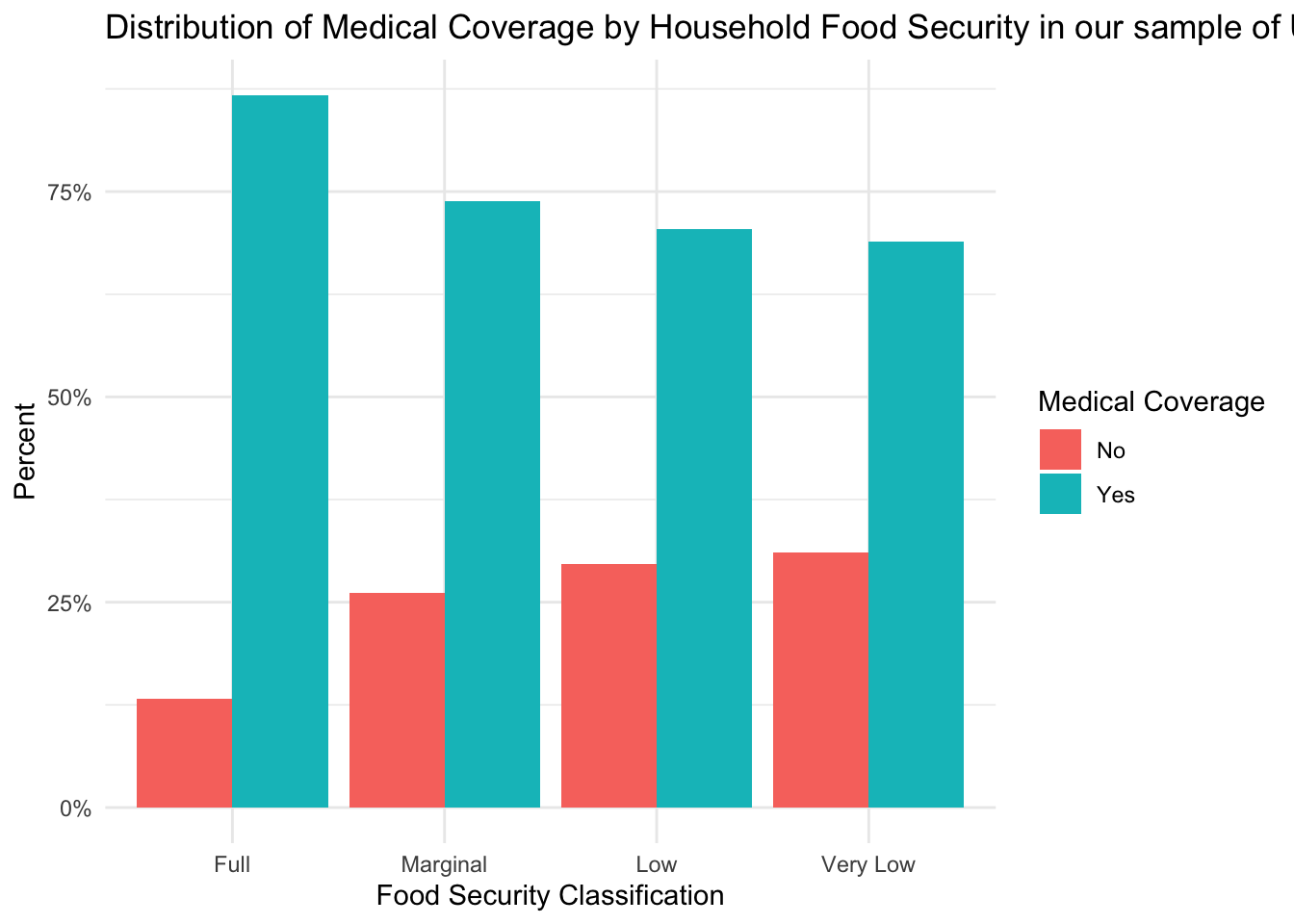
From this figure, we can see that over 75% of subjects in each food security group have some form of medical coverage. It is important to note, however, that there is a trend for decreasing insurance coverage as the level of food insecurity increases. Given that a lack of insurance might decrease healthcare-seeking behaviors, insurance coverage could be an important factor to consider when interpreting the results of our analyses.
Our goals for this exploratory data analysis will be to better understand health outcomes in our sample of U.S. adults.
The primary research questions that we will explore are:
Does the prevalence of metabolic health conditions, such as high blood pressure, high cholesterol, diabetes, and obesity, differ by food security levels in our sample of U.S. adults?
Do levels of inflammatory factors, such as C-reactive protein, differ by food security levels in our sample of U.S. adults? If so, could inflammatory factors help explain the relationship between food security and health outcomes?
The secondary research question that I would like to explore is:
As mentioned in the introduction to the project, many research studies that have explored health outcomes in food-insecure individuals have focused on metabolic conditions (conditions that are risk factors for cardiovascular diseases), such as obesity and diabetes. Therefore, for our analysis, we will also look at how the proportion of subjects diagnosed with metabolic conditions differs by food security status.
The first health outcome that we will explore is obesity, which is a disorder that is characterized by an excess of body fat. Body Mass Index can be used to diagnose obesity, and the BMI classifications are defined as follows:
Below, we see the BMI distribution for each food security group.
sample %>%
ggplot(aes(x = hh_food_security, y = bmi)) +
geom_boxplot() +
theme_minimal() +
labs(
title = "BMI Distribution by Food Security Status",
x = 'Food Security',
y = 'BMI'
)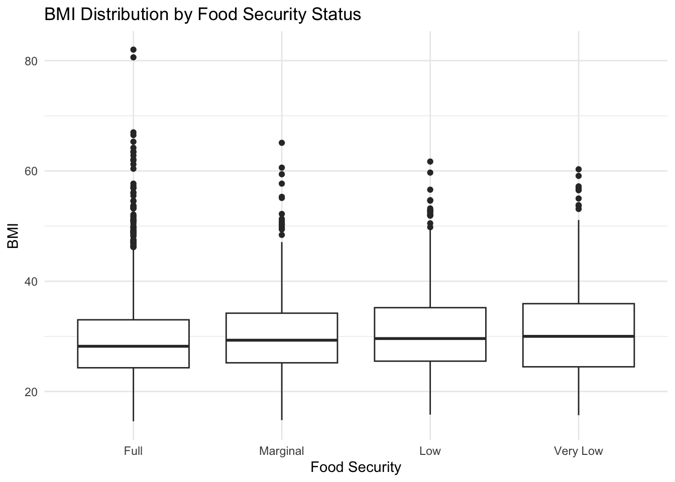
It is interesting to see that all groups appear to have a median BMI value that would be classified as overweight (BMI >= 25), and the very low food-secure group has a median BMI that appears to be classified as obese.
If we look at the percentage of subjects in each food security group by BMI classification, a similar pattern emerges.
counts_by_fs <- sample %>%
group_by(hh_food_security) %>%
summarize(total = n())
sample %>%
mutate(bmi_class = case_when(
bmi < 18.5 ~ 'Underweight',
bmi >= 18.5 & bmi <= 24.9 ~ 'Normal',
bmi >= 25.0 & bmi <= 29.9 ~ 'Overweight',
bmi >= 30 ~ 'Obese')) %>%
mutate(bmi_class = factor(bmi_class, levels = c('Underweight', 'Normal', 'Overweight', 'Obese'))) %>%
group_by(bmi_class, hh_food_security) %>%
summarize(count = n()) %>%
left_join(counts_by_fs, by = 'hh_food_security') %>%
mutate(percent = count/total) %>%
ggplot(aes(x = hh_food_security, y = percent, fill = bmi_class)) +
geom_col(position='dodge') +
theme_minimal() +
scale_y_continuous(labels = scales::percent) +
labs(
title = 'BMI Classification by Food Security Group',
x = 'Food Security',
y = 'Percent',
fill = 'BMI Classification'
)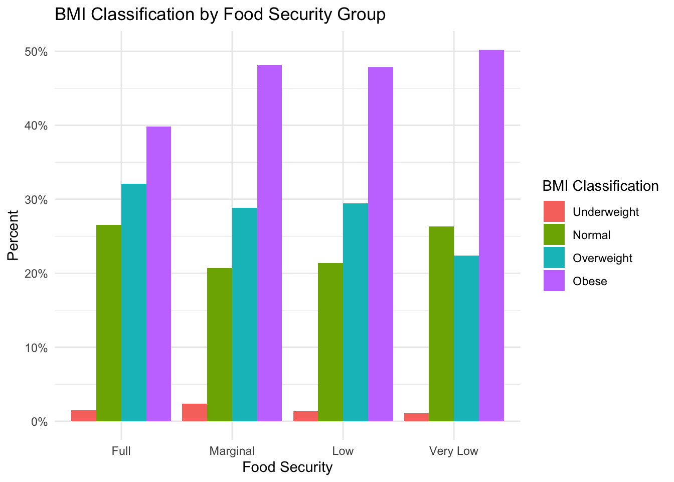
Here, we see that the predominant BMI classification across all groups is “Obese”; however, the percentage of obese subjects in the “Marginal”, “Low” and “Very Low’ food-secure groups is larger than in the”Full” food-secure group. This suggests that, similar to the literature, food insecurity could be associated with higher rates of obesity in our sample.
Additionally, we are interested in understanding how levels of diabetes differ by food security status in our sample.
counts_by_fs <- sample %>%
group_by(hh_food_security) %>%
summarize(total = n())
sample %>%
group_by(diabetes, hh_food_security) %>%
summarize(count = n()) %>%
left_join(counts_by_fs, by = 'hh_food_security') %>%
mutate(percent = count/total) %>%
ggplot(aes(x = hh_food_security, y = percent, fill = diabetes)) +
geom_col(position='dodge') +
theme_minimal() +
scale_y_continuous(labels = scales::percent) +
labs(
title = 'Diabetes Classification by Food Security Group',
x = 'Food Security',
y = 'Percent',
fill = 'Diabetes'
)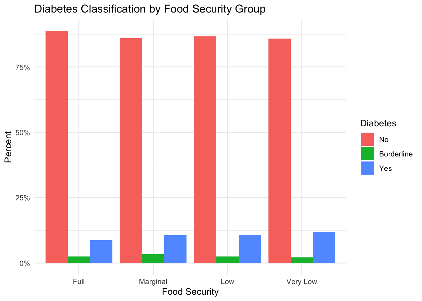
In the figure above, we see that the vast majority of subjects in our sample have never been diagnosed with diabetes. However, if we compare the percentage of subjects who have diabetes between the different groups, we see a slightly higher percentage of subjects in the food-insecure groups with diabetes than in the fully food-secure group. This suggests a possible relationship between food security and diabetes in our sample.
Another metabolic condition of interest is high blood pressure. Below we see that proportion of subjects diagnosed with high blood pressure for each food security group.
counts_by_fs <- sample %>%
group_by(hh_food_security) %>%
summarize(total = n())
sample %>%
group_by(high_bp, hh_food_security) %>%
summarize(count = n()) %>%
left_join(counts_by_fs, by = 'hh_food_security') %>%
mutate(percent = count/total) %>%
ggplot(aes(x = hh_food_security, y = percent, fill = high_bp)) +
geom_col(position='dodge') +
theme_minimal() +
scale_y_continuous(labels = scales::percent) +
labs(
title = 'Blood Pressure Status by Food Security Group',
x = 'Food Security',
y = 'Percent',
fill = 'High Blood Pressure'
)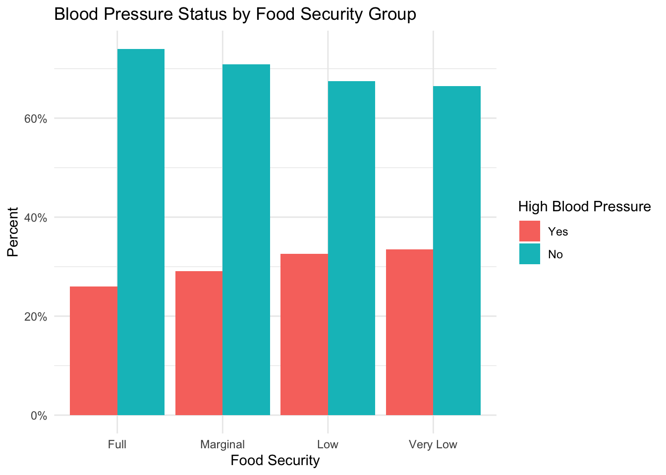
This figure shows a trend towards a larger percentage of subjects with high blood pressure as food insecurity level increases.
Finally, we explore how diagnosed high cholesterol differs by food insecurity level.
counts_by_fs <- sample %>%
group_by(hh_food_security) %>%
summarize(total = n())
sample %>%
group_by(high_cholesterol, hh_food_security) %>%
summarize(count = n()) %>%
left_join(counts_by_fs, by = 'hh_food_security') %>%
mutate(percent = count/total) %>%
ggplot(aes(x = hh_food_security, y = percent, fill = high_cholesterol)) +
geom_col(position='dodge') +
theme_minimal() +
scale_y_continuous(labels = scales::percent) +
labs(
title = 'Cholesterol Status by Food Security Group',
x = 'Food Security',
y = 'Percent',
fill = 'High Cholesterol'
)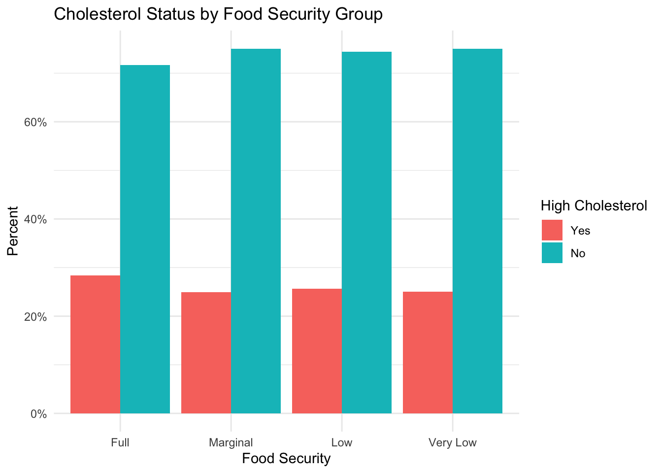
Contrary to the previous metabolic conditions, it appears that there is a higher percentage of subjects with high cholesterol in the fully food-secure group than in the groups experiencing some form of food insecurity. For a future analysis, it would be interesting to see how dietary habits impact this finding.
Overall, the results of this exploration suggest that individuals experiencing food insecurity could be at greater risk for developing obesity, diabetes, and high blood pressure.
Because inflammation has been known to predict metabolic conditions and cardiovascular disease, we are also interested in knowing if there is a difference in CRP level by food security group.
sample %>%
ggplot(aes(x = hh_food_security, y = crp_mgL)) +
geom_boxplot()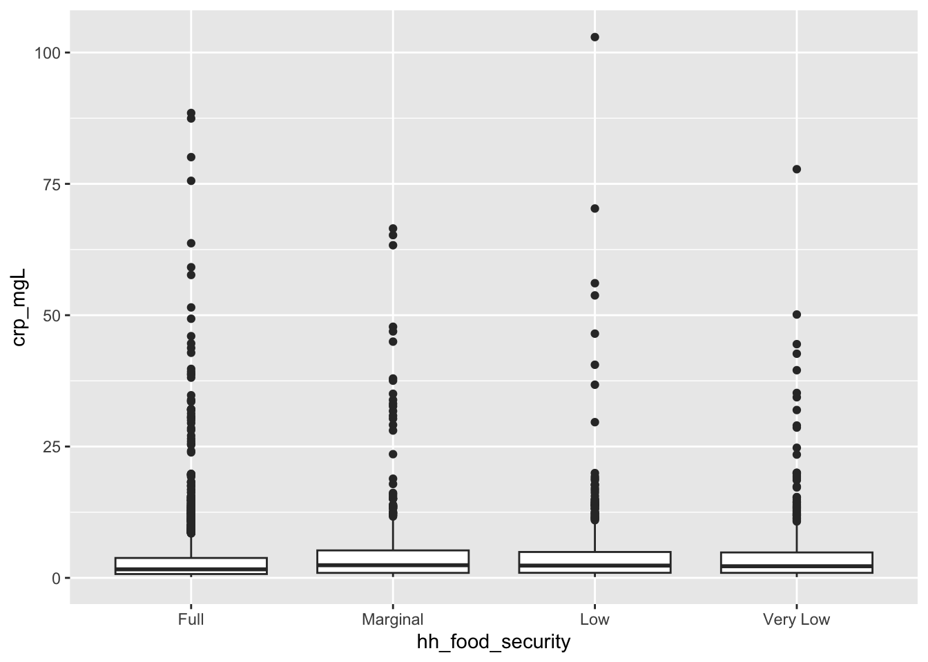
From the box plots above, we can see that food-insecure groups appear to have higher CRP levels than fully food-secure individuals. Some descriptive statistics are shown in the table below.
sample %>%
group_by (hh_food_security) %>%
summarize(
mean_crp = mean(crp_mgL),
std_dev_crp = sd(crp_mgL),
median_crp = median(crp_mgL)
)We can also analyze CRP based on groupings used to determine elevated risk of cardiovascular disease. The classifications for CRP are:
sample <- sample %>%
mutate(crp_group = case_when(
crp_mgL < 1 ~ 'Low',
crp_mgL >= 1 & crp_mgL <= 3 ~ 'Moderate',
crp_mgL > 3 ~ 'High'
),
crp_group = factor(crp_group, levels = c('Low', 'Moderate', 'High')))
sample %>%
group_by(crp_group, hh_food_security) %>%
summarize(count = n()) %>%
left_join(counts_by_fs, by = 'hh_food_security') %>%
mutate(percent = count/total) %>%
ggplot(aes(x = hh_food_security, y = percent, fill = crp_group)) +
geom_col(position='dodge') +
theme_minimal() +
scale_y_continuous(labels = scales::percent) +
labs(
title = 'CRP Risk Classification by Food Security Group',
x = 'Food Security',
y = 'Percent',
fill = 'CRP Risk'
)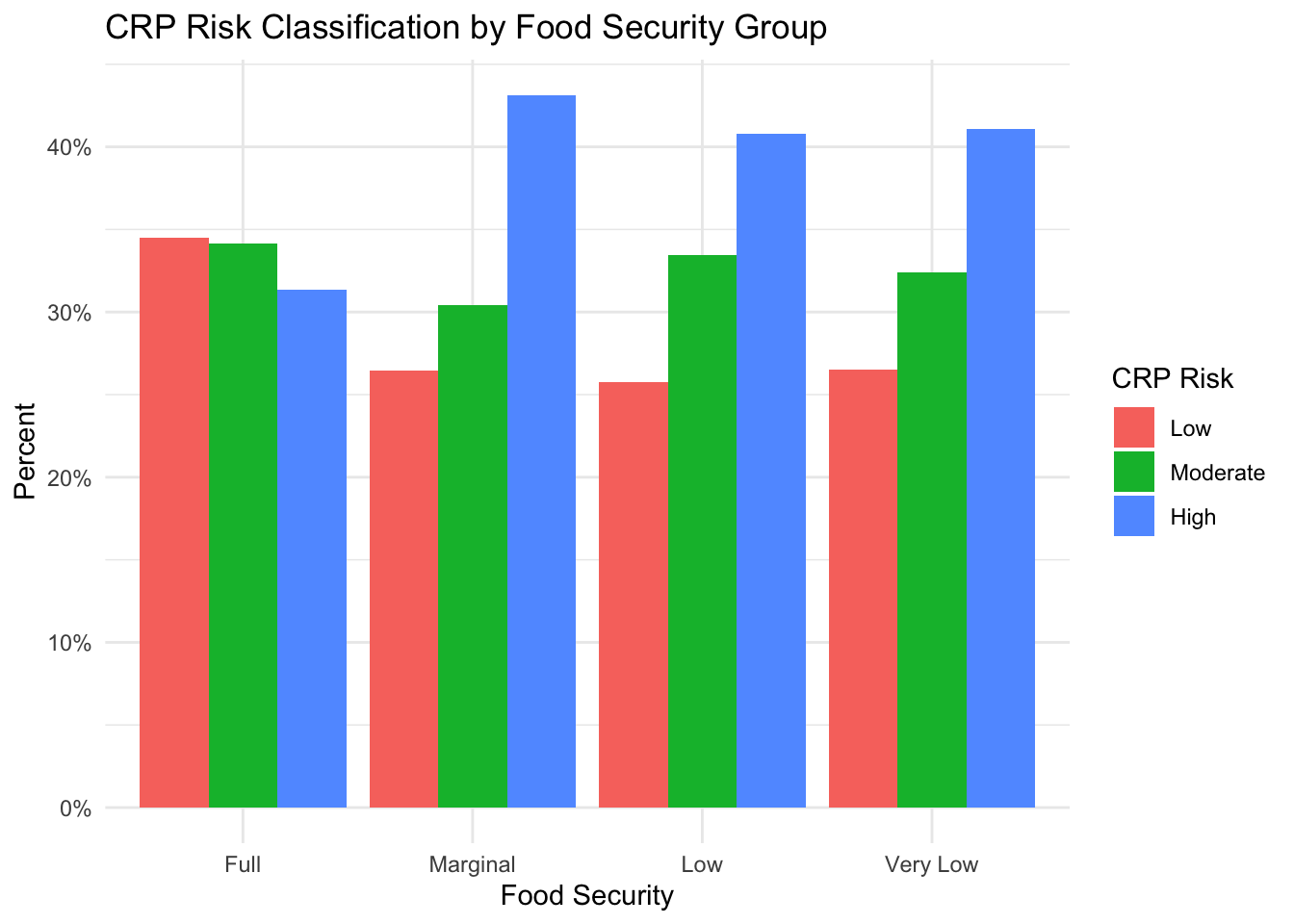
From this figure, we can see that the percentage of individuals with high-risk CRP levels is higher in groups with some level of food insecurity than the group with full food security. However, it is interesting to see that the highest percentage is in the ‘Marginal’ food-secure group.
Note: given the number of outliers on the boxplot, we might want to consider investigating why those CRP values are so high (e.g. medical conditions such as arthritis, recent infection, etc.)
Finally, given that we have shown an increased percentage of individuals in food-insecure groups with obesity, diabetes, and high blood pressure, and we have also shown elevated levels of CRP in food-insecure groups, we can now explore if the pattern of disease risk changes once we subset the data by CRP level.
Obesity
Below we see the exact same graph from above, but now, we facet the data by CRP risk group. (Note: in this case, the sum of each food security group is 100%)
sample %>%
mutate(bmi_class = case_when(
bmi < 18.5 ~ 'Underweight',
bmi >= 18.5 & bmi <= 24.9 ~ 'Normal',
bmi >= 25.0 & bmi <= 29.9 ~ 'Overweight',
bmi >= 30 ~ 'Obese')) %>%
mutate(bmi_class = factor(bmi_class, levels = c('Underweight', 'Normal', 'Overweight', 'Obese'))) %>%
group_by(bmi_class, hh_food_security, crp_group) %>%
summarize(count = n()) %>%
left_join(counts_by_fs, by = 'hh_food_security') %>%
mutate(percent = count/total) %>%
ggplot(aes(x = hh_food_security, y = percent, fill = bmi_class)) +
geom_col(position='dodge') +
facet_grid(vars(crp_group)) +
theme_minimal() +
scale_y_continuous(labels = scales::percent) +
labs(
title = 'BMI Classification by Food Security Group and CRP Level',
x = 'Food Security',
y = 'Percent',
fill = 'BMI Classification'
)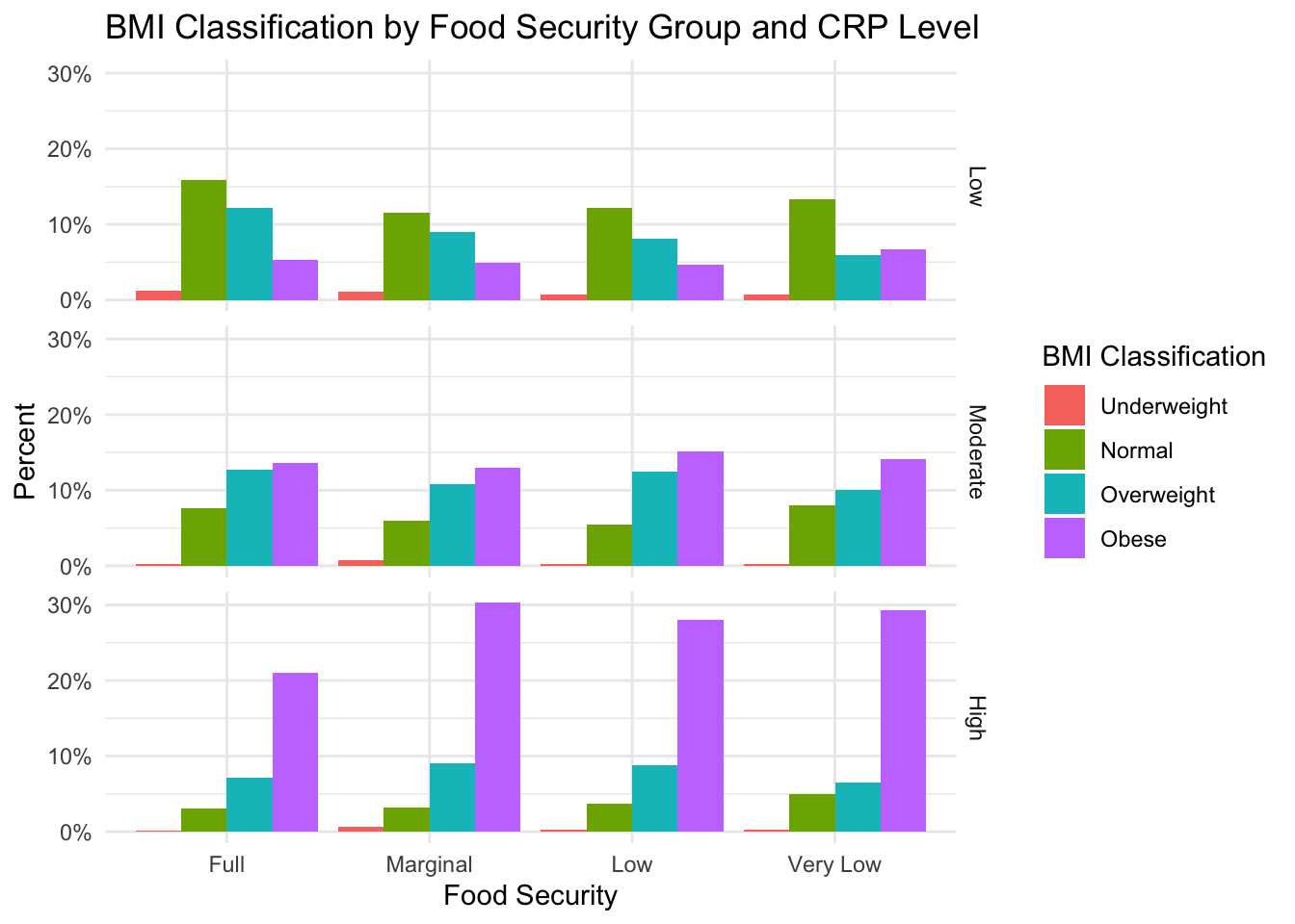
Based on this figure, we can see that obesity appears to be most prevalent in the high-risk CRP group. However, this pattern applies across food-security groups, so it is not likely that CRP levels fully explain the relationship between obestiy and food insecurity.
Diabetes
A similar plot is shown for diabetes.
sample %>%
group_by(diabetes, hh_food_security, crp_group) %>%
summarize(count = n()) %>%
left_join(counts_by_fs, by = 'hh_food_security') %>%
mutate(percent = count/total) %>%
ggplot(aes(x = hh_food_security, y = percent, fill = diabetes)) +
geom_col(position='dodge') +
facet_grid(rows = vars(crp_group)) +
theme_minimal() +
scale_y_continuous(labels = scales::percent) +
labs(
title = 'Diabetes Classification by Food Security Group and CRP Level',
x = 'Food Security',
y = 'Percent',
fill = 'Diabetes'
)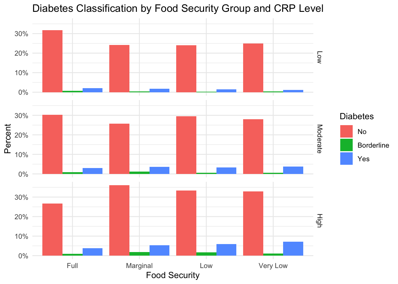
Similarly, CRP level does not seem to explain the relationship between diabetes and food insecurity.
High Blood Pressure
sample %>%
group_by(high_bp, hh_food_security, crp_group) %>%
summarize(count = n()) %>%
left_join(counts_by_fs, by = 'hh_food_security') %>%
mutate(percent = count/total) %>%
ggplot(aes(x = hh_food_security, y = percent, fill = high_bp)) +
geom_col(position='dodge') +
facet_grid(rows = vars(crp_group)) +
theme_minimal() +
scale_y_continuous(labels = scales::percent) +
labs(
title = 'Blood Pressure Classification by Food Security Group and CRP Level',
x = 'Food Security',
y = 'Percent',
fill = 'High Blood Pressure'
)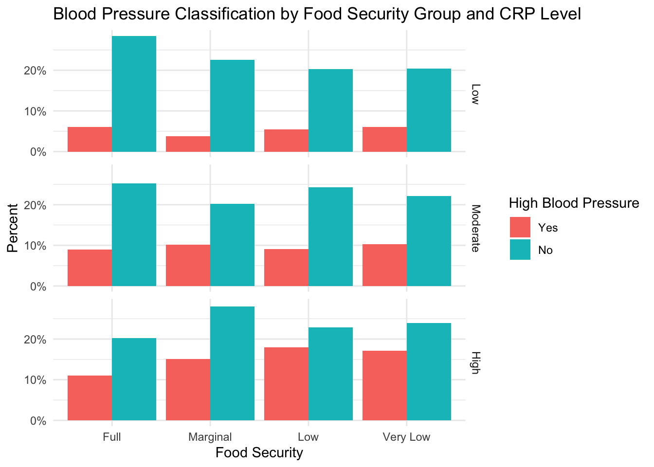
CRP level does not seem to explain the relationship between high blood pressure and food insecurity
Psychological impact of food insecurity. One limitation of this dataset is that it does not allow us to quantify the difficulty that food insecurity imposes on individual subjects’ lives. Because stress is known to exacerbate many health outcomes, it would be interesting to understand how the psychological distress associated with food insecurity impacts inflammation.
Inequality of food security group sizes. As found in the U.S. population, our study sample exhibits a class imbalance between people who are fully food-secure and the groups experiencing some form of food insecurity. To increase confidence in our findings, we might wish to increase the number of food insecure individuals in our sample. Additionally, the unequal sample sizes mean that I used percentages for all of my comparisons. Percentages can vary greatly by sample size, which is another limitation.
Visualizing mediation effects. To see if CRP levels could explain the relationship between health outcomes and food security group, I used bar plots faceted by CRP level. It is possible that this was not the right approach to study this relationship. A more thorough approach might be to conduct a statistical analysis, where CRP level can be a mediator.
Berkowitz, S.A., Baggett, T.P., Wexler, D.J., Huskey, K.W., & Wee, C.C. (2013). Food insecurity and metabolic control among U.S. adults with diabetes. Diabetes Care, 36, 3093–9.
Bermudez-Millan, A., Wagner, J.A., Feinn, R.S., Segura-Perez, S., Damio, G., Chhabra, J., & Perez-Escamilla, R. (2019). Inflammation and Stress Biomarkers Mediate the Association between Household Food Insecurity and Insulin Resistance among Latinos with Type 2 Diabetes, Journal of Nutrition, 982-988.
Gowda, C., Hadley, C., & Aiello, A.E. (2012). The Association Between Food Insecurity and Inflammation in the US Adult Population. American Journal of Public Health, 102(8), 1579-1586.
Harvard Health Publishing. (2017). C-Reactive Protein test to screen for heart disease: Why do we need another test? Link
Hernandez, D.C., Reesor, L.M, & Murillo R. (2017). Food insecurity and adult overweight/obesity: gender and race/ethnic disparities. Appetite 117, 373–8.
National Center for Health Statistics (2020). National Health and Nutrition Examination Survey Data. U.S. Department of Health and Human Services, Centers for Disease Control and Prevention.
R Core Team. (2023). R: A Language and Environment for Statistical Computing. R Foundation for Statistical Computing. https://www.R-project.org/
United States Department of Agriculture, Economic Research Service. (2023). Key statistics & graphics. Link
Zierath, R., Clagget, B., Hall, M.E., Correa, A., Barber, S., Gao, Y., Talegawkar, S., Ezekwe, E.I., Tucker, K., Diez-Rouz, A.V., Sims, M. & Shah, A.M. (2023). Measures of Food Inadequacy and Cardiovascular Disease Risk in Black Individuals in the US From the Jackson Heart Study. JAMA Network Open.