Challenge 10

purrr

library(tidyverse)
library(here)
library(readr)
library(stringr)
library(purrr)
library(glue)

knitr::opts_chunk$set(echo = TRUE, warning=FALSE, message=FALSE)

Challenge Overview

Use purrr with a function to perform some data science task. What this task is is up to you. It could involve computing summary statistics, reading in multiple datasets, running a random process multiple times, or anything else you might need to do in your work as a data analyst. You might consider using purrr with a function you wrote for challenge 9.

Implementation

For this challenge, I will use the SNL dataset that was used in Challenge 8. The main focus will be to use the purrr package to accomplish two tasks:

1. Import multiple datasets at once

2. Fill-in missing rows

Goal 1: Read in multiple data files

To begin, I am interested in learning how purrr can be used to read in multiple data files at the same time. To do this, we will begin by creating a list of the file names corresponding to the SNL dataset. This can be done by using list.files() to view all files in the _data folder and using purrr::keep() with stringr::str_detect to filter to only file names containing 'snl_'.

# list all files
# use purrr::keep() to only keep the file names containing snl_
dir_path <- here('posts', '_data')
snl_files <- keep(list.files(dir_path), ~str_detect(.x, 'snl_'))

snl_files

[1] "snl_actors.csv"  "snl_casts.csv"   "snl_seasons.csv"

Next, we will import each of the data frames at once. To do this, we will use the purrr::map() function along with readr::read_csv to save each data frame as an element of an R list. As a pre-processing step, we will also use purrr::map() to convert the individual file names into full file paths.

# first we will use purrr::map() to prepend the `_data` directory to each file name
snl_files <- map(snl_files, ~glue("{dir_path}/{.x}"))

# then, we read in each df to a list
snl_df_list <- snl_files %>%
  map(read_csv)

We can then easily, filter the list to get the separate data frames, which can be joined in the same way as Challenge 8.

actors <- snl_df_list[[1]]
cast <- snl_df_list[[2]]
seasons <- snl_df_list[[3]]

joined <- cast %>%
  left_join(actors, by = 'aid') %>%
  left_join(seasons, by = 'sid', suffix = c('_actor', '_season'))

joined

Goal 2: Fill in “Missing” Rows

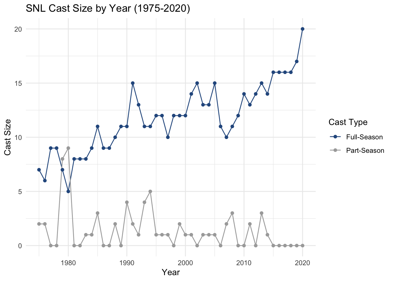
When working on the analysis portion of Challenge 8, I noticed that, when computing summary statistics, if a combination of year and cast_type did not appear in the raw data table, the point would be missing from the graph. In the figure below, this is illustrated by the line for Part-Season missing several points on the graph.

joined %>%
  # limit to cast members
  filter(type == 'cast') %>%
  # create a full-time cast indicator var
  mutate(full_time_cast = factor(ifelse(season_fraction == 1, 'Full-Season', 'Part-Season'))) %>%
  # get the count of actors for each year and cast type
  distinct(year, aid, full_time_cast) %>%
  group_by(year, full_time_cast) %>%
  summarize(count = n()) %>%
  # plot the change over time
  ggplot(aes(x = year, y = count, color = full_time_cast)) +
  geom_line() +
  geom_point() +
  theme_minimal() +
  labs(title = 'SNL Cast Size by Year (1975-2020)',
    x = 'Year',
    y = 'Cast Size',
    color = 'Cast Type') +
  scale_color_manual(values = c('#2B598E', 'darkgrey'))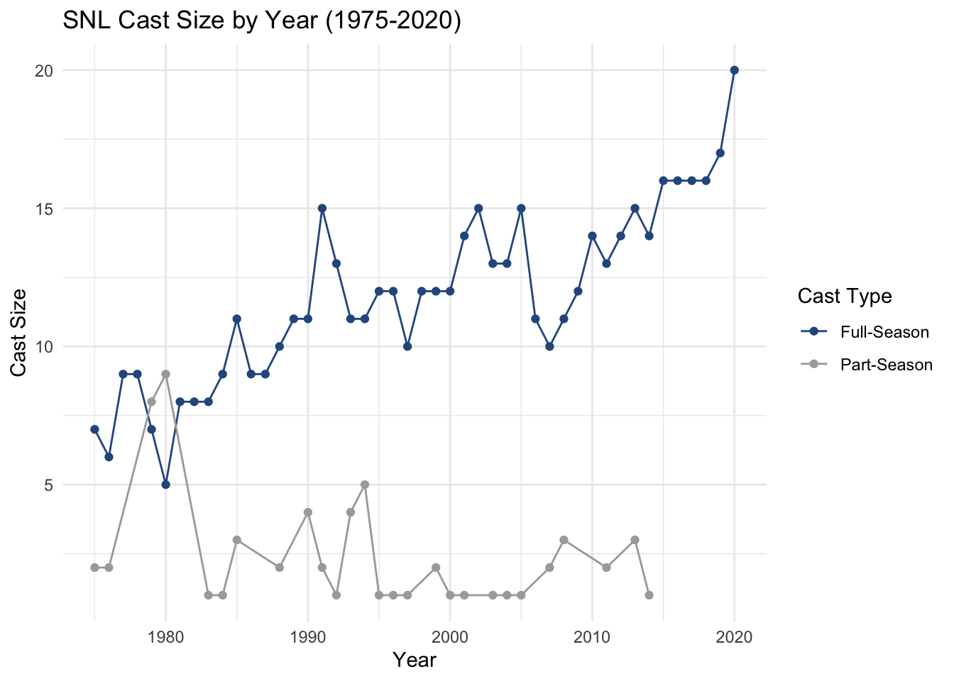

When computing the summary statistics (where we are essentially counting the number of rows when grouping by year and cast_type), if there are 0 rows, we would the count to be 0 instead of just not appearing in the data. We can use purrr to help us fill in these rows.

First, we use purrr::cross_df() to create a data frame containing all possible combinations of year and cast_type. Because there are 46 years covered by the dataset, we should expect to see 92 rows in the resulting data frame–which we do!

# create vector of distinct years
years = joined %>% 
  distinct(year) %>% 
  pull(year)

# create a vector of distinct cast types
cast_types = c('Full-Season', 'Part-Season')

# use purrr::cross_df() to create a df containing all possible combos of year and cast type. 
combos <- list(year = years, cast_type = cast_types)
year_cast_combos <- cross_df(combos) %>%
  arrange(year, cast_type)

year_cast_combos

Now, we can construct a data frame (counts) that contains the counts of cast members by year and cast_type. The counts data frame can be left-joined to the year_cast_combos data frame. If a year-cast_type combination was missing from the original data frame, it will have an NA count.

# get summary counts df
counts <- joined %>%
  # limit to cast members
  filter(type == 'cast') %>%
  # create a full-time cast indicator var
  mutate(cast_type = factor(ifelse(season_fraction == 1, 'Full-Season', 'Part-Season'))) %>%
  # get the count of actors for each year and cast type
  distinct(year, aid, cast_type) %>%
  group_by(year, cast_type) %>%
  summarize(count = n())

# start with all possible years
full_counts <- year_cast_combos %>%
  # join the published data
  left_join(counts, c('year', 'cast_type'))

full_counts

The NA values can then be filled with 0. Now, when we re-plot the figure, we see that the same number of points appear for both Full-Time and Part-Time cast.

full_counts %>%
  mutate(count = replace_na(count, 0)) %>% 
  ggplot(aes(x = year, y = count, color = cast_type)) +
  geom_line() +
  geom_point() +
  theme_minimal() +
  labs(title = 'SNL Cast Size by Year (1975-2020)',
    x = 'Year',
    y = 'Cast Size',
    color = 'Cast Type') +
  scale_color_manual(values = c('#2B598E', 'darkgrey'))