Challenge 8: Joining Data

Joining tables from the SNL dataset

library(tidyverse)
library(here)
library(lubridate)
library(ggplot2)

knitr::opts_chunk$set(echo = TRUE, warning=FALSE, message=FALSE)

Read in data

For this challenge, I will be using the SNL dataset.

actors <- read_csv(here('posts', '_data', 'snl_actors.csv'))
casts <-  read_csv(here('posts', '_data', 'snl_casts.csv'))
seasons <-  read_csv(here('posts', '_data', 'snl_seasons.csv'))

Briefly describe the data

The SNL data set is comprised of three tables: actors, casts, and seasons.

Actors

The actors table contains data to describe the different actors from SNL. This table contains data, such as their URL, type of actor on the show (e.g. cast, crew, guest), and gender. Each of the 2306 rows is uniquely defined using an identification variable named aid.

actors

Casts

The casts table provides information about the casts of the different seasons. This table contains data to match an actor to a season and descriptive information about their time on the season, such as their first and last episode dates, if they were an anchor for “Weekend Update”, and the number of episodes they acted on. Each of the 614 rows is uniquely identified by the actor id (aid) and season id (sid).

casts

Seasons

The seasons table provides information about 46 different seasons of SNL, such as the year, dates of the first and last episodes, and number of episodes.

seasons

Tidy Data (as needed)

In its raw form, the data is already tidy, so no pivoting will be needed. However, after reviewing the data, there are still some cleaning steps that we should take.

First, we will mutate the data so that all of the date columns are properly formatted as dates.

# Casts table
cast_date_cols <- casts %>%
  select(contains('epid')) %>% 
  colnames()

casts <- casts %>%
  mutate(across(cast_date_cols, ymd))

glimpse(casts)

Rows: 614
Columns: 8
$ aid             <chr> "A. Whitney Brown", "A. Whitney Brown", "A. Whitney Br…
$ sid             <dbl> 11, 12, 13, 14, 15, 16, 5, 39, 40, 41, 42, 45, 46, 21,…
$ featured        <lgl> TRUE, TRUE, TRUE, TRUE, TRUE, TRUE, TRUE, TRUE, TRUE, …
$ first_epid      <date> 1986-02-22, NA, NA, NA, NA, NA, 1980-04-09, 2014-01-1…
$ last_epid       <date> NA, NA, NA, NA, NA, NA, NA, NA, NA, NA, NA, NA, NA, N…
$ update_anchor   <lgl> FALSE, FALSE, FALSE, FALSE, FALSE, FALSE, FALSE, FALSE…
$ n_episodes      <dbl> 8, 20, 13, 20, 20, 20, 5, 11, 21, 21, 21, 18, 17, 20, …
$ season_fraction <dbl> 0.4444444, 1.0000000, 1.0000000, 1.0000000, 1.0000000,…

# Seasons table
season_date_cols <- seasons %>%
  select(contains('epid')) %>% 
  colnames()

seasons <- seasons %>%
  mutate(across(season_date_cols, ymd))

glimpse(seasons)

Rows: 46
Columns: 5
$ sid        <dbl> 1, 2, 3, 4, 5, 6, 7, 8, 9, 10, 11, 12, 13, 14, 15, 16, 17, …
$ year       <dbl> 1975, 1976, 1977, 1978, 1979, 1980, 1981, 1982, 1983, 1984,…
$ first_epid <date> 1975-10-11, 1976-09-18, 1977-09-24, 1978-10-07, 1979-10-13…
$ last_epid  <date> 1976-07-31, 1977-05-21, 1978-05-20, 1979-05-26, 1980-05-24…
$ n_episodes <dbl> 24, 22, 20, 20, 20, 13, 20, 20, 19, 17, 18, 20, 13, 20, 20,…

Next, it appears that the gender column from actors might have some values that would be better coded as NA. Given that the gender classification appears to be binary, we will classify andy and unknown as NA.

actors %>%
  group_by(gender) %>%
  tally()

actors <- actors %>%
  mutate(gender = ifelse(gender %in% c('andy', 'unknown'), NA, gender))

actors %>%
  group_by(gender) %>%
  tally()

Finally, we will convert all categorical variables in the tables to factors.

actors <- actors %>%
  mutate(gender = factor(gender, levels = c('male', 'female')))

glimpse(actors)

Rows: 2,306
Columns: 4
$ aid    <chr> "Kate McKinnon", "Alex Moffat", "Ego Nwodim", "Chris Redd", "Ke…
$ url    <chr> "/Cast/?KaMc", "/Cast/?AlMo", "/Cast/?EgNw", "/Cast/?ChRe", "/C…
$ type   <chr> "cast", "cast", "cast", "cast", "cast", "guest", "guest", "cast…
$ gender <fct> female, male, NA, male, male, NA, male, female, male, male, fem…

Join Data

Now, we will use the unique identification columns to join the three tables into a single table. Because we do not want to lose any data, we will use a left join. When joining our tables, we will start with casts. This table includes both aid and sid, which will make it easy to join the other two tables. We will also specify a suffix for any variable names that overlap between the tables.

With a left_join, we would expect to see a table with 614 rows and 15 columns. (Note: because we join on aid and sid, those columns only appear in the data once.)

joined <- casts %>%
  left_join(actors, by = 'aid') %>%
  left_join(seasons, by = 'sid', suffix = c('_actor', '_season'))

joined

From the data frame above, we can see that our resulting joined table matches our expected dimensions!

Analysis

For our analysis of the data, we will explore how the size and composition of the SNL cast has changed over time. From the table below, we can see that there is only one season of SNL for each year, so we will use year as our time variable.

joined %>%
  distinct(sid, year) %>%
  group_by(sid) %>%
  summarize(n_years = n()) %>%
  arrange(desc(n_years))

First, we will explore how the size of the full-time and part-time cast has changed over time. To do this, we will first construct a variable, where Full-Season means that an actor appeared in all episodes of a season and Part-Season means that an actor only appeared in some episodes. We will then use group_by and summarize to obtain counts of actors per group. We will use a connected scatter plot to show how the counts vary over group and time.

joined %>%
  # limit to cast members
  filter(type == 'cast') %>%
  # create a full-time cast indicator var
  mutate(full_time_cast = factor(ifelse(season_fraction == 1, 'Full-Season', 'Part-Season'))) %>%
  # get the count of actors for each year and cast type
  distinct(year, aid, full_time_cast) %>%
  group_by(year, full_time_cast) %>%
  summarize(count = n()) %>%
  # plot the change over time
  ggplot(aes(x = year, y = count, color = full_time_cast)) +
  geom_line() +
  geom_point() +
  theme_minimal() +
  labs(title = 'SNL Cast Size by Year (1975-2020)',
    x = 'Year',
    y = 'Cast Size',
    fill = 'Cast Type') +
  scale_color_manual(values = c('#2B598E', 'darkgrey'))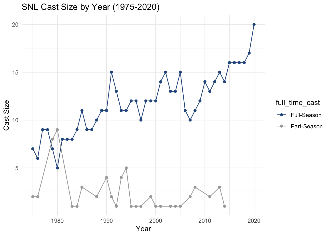

From the graph above, we can see that there is an increasing trend in the number of full-season members on SNL. Since 1980, the number of part-season cast members has remained fairly low.

Given that the number of full-season cast members has been increasing since 1975, we can also explore how the gender composition of the cast has changed over time. For this analysis, we will use group_by and summarize to calculate the percentage of males and females on the cast, and we will use a stacked bar plot to visualize the results. In this case, because the percentage for each year sums to 100%, a stacked bar plot seems to be a fairly easy way to see differences in the groups.

totals_by_year <- joined %>%
  filter(type == 'cast', season_fraction == 1, !is.na(gender)) %>%
  distinct(year, aid) %>%
  group_by(year) %>%
  summarize(total_count = n())
  
joined %>%
  filter(type == 'cast', season_fraction == 1, !is.na(gender)) %>%
  mutate(gender = ifelse(gender == 'male', 'M', 'F')) %>%
  distinct(year, aid, gender) %>%
  group_by(year, gender) %>%
  summarize(count = n()) %>%
  left_join(totals_by_year, by = 'year') %>%
  mutate(pct = round(count / total_count, 1)) %>%
  ggplot(aes(x = year, y = pct, fill = gender)) +
  geom_col() +
  labs(title = 'Gender Composition of SNL Cast (1975-2020)',
    x = 'Year',
    y = 'Percent',
    fill = 'Gender') + 
  theme_minimal() + 
  scale_y_continuous(labels = scales::percent) + 
  # color scales for gender
  # https://blog.datawrapper.de/gendercolor/
  scale_fill_manual(values = c('#EB9347', '#5AABB9'))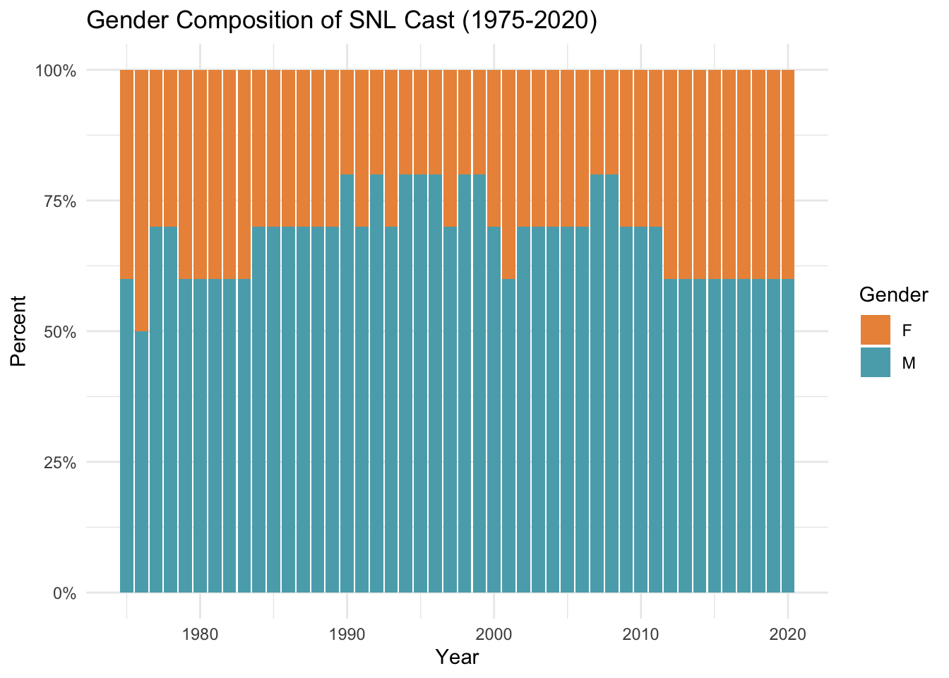

From this graph, we can see that across time, males have made up a larger percentage of the SNL cast. In recent years, however, the percentage of males has been fairly stable at ~60%, which is a decrease from previous years.