Code
library(tidyverse)
library(here)
library(haven)
library(glue)
library(ggplot2)

knitr::opts_chunk$set(echo = TRUE)library(tidyverse)
library(here)
library(haven)
library(glue)
library(ggplot2)
knitr::opts_chunk$set(echo = TRUE)For this homework, I have chosen to to explore data from the National Health and Nutrition Examination Survey (NHANES), an annual survey conducted by the National Center for Health Statistics (NCHS) that assesses the health and nutritional status of adults and children. The population sampled from NHANES is designed to be representative of the United States population, and data is collected through both comprehensive interviews and laboratory examinations.
NHANES data is divided into five main categories:
Demographics Data: Demographic and socioeconomic information about study participants, such as country of birth, education level, gender, race, and age.
Dietary Data: Information about supplement-use and food/nutritional intake
Examination Data: Information that comes from a physical examination, such as blood pressure, anthropomorphic measures (e.g. weight), and oral health.
Laboratory Data: Information that comes from serum lab tests, such as blood lipids, liver proteins, and many others.
Questionnaire Data: Information that comes from an interview, including personal and family health history, medication use, physical activity, and many others.
Each category contains many data tables, each of which corresponds to a specific topic. For example, the questionnaire data contains 39 separate data files corresponding to different topics from the questionnaire. Each of the tables can be joined using the SEQN column, which corresponds to the ID for an individual participant.
The website for NHANES currently has data dating back to 1999 available to the public, but for this analysis, I will focus on the batch of data collected from January 2017 to March 2020 (pre-pandemic data).
The NHANES data files are designed to be analyzed via SAS, and therefore, they are only available in .XPT format. To read-in these files using R, we can use the read_xpt() function from the haven package.
For the final project, I know that I would like to work with NHANES data but am still exploring possible topics. One possible topic would be to explore stress as an inflammatory condition. Therefore, as a starting point, I will read-in some data files that could possibly be used for this analysis:
data_dir <- 'hw_2_datafiles_jocelyn_lutes'
base_path <- here('posts', data_dir)

read_data_from_base <- function(path) {
  return(read_xpt(glue('{base_path}/{path}')))
}

demo <- read_data_from_base('P_DEMO.XPT')
crp <- read_data_from_base('P_HSCRP.XPT')
food_security <- read_data_from_base('P_FSQ.XPT')
mental_health <- read_data_from_base('P_DPQ.XPT')The demographics dataset provides demographic information for 15560 study participants. The raw dataset contains 29 columns, but we will limit the data to only include the identifier column and 5 columns of interest:
demo_clean <- demo %>%
  select(
    id = SEQN,
    age = RIDAGEYR,
    gender = RIAGENDR,
    race = RIDRETH3,
    education_level = DMDEDUC2,
    income_poverty_ratio = INDFMPIR
    )

names(demo_clean)
[1] "id" "age" "gender"
[4] "race" "education_level" "income_poverty_ratio"head(demo_clean)As shown in the head() above, the NHANES data is entered according to a code. Therefore, for easier understanding, we will recode categorical data from numeric values to factors.
# recode values
demo_clean <- demo_clean %>%
  mutate(
    gender = case_when(
      gender == 1 ~ 'M',
      gender == 2 ~ 'F',
      gender == '.' ~ NA),
    race = case_when(
      race == 1 ~ 'Mexican American',
      race == 2 ~ 'Other Hispanic',
      race == 3 ~ 'Non-Hispanic White',
      race == 4 ~ 'Non-Hispanic Black',
      race == 7 ~ 'Other Race',
      race == 6 ~ 'Non-Hispanic Asian',
      race == '.' ~ NA
    ),
    education_level = case_when(
      education_level %in% c(1, 2) ~ 'Less than HS',
      education_level == 3 ~ 'HS',
      education_level == 4 ~ 'Some College',
      education_level == 5 ~ 'College Grad or Above',
      education_level %in% c(7, 9) ~ NA,
      education_level == '.' ~ NA
      )
)

# convert categorical vars to factors
demo_clean <- demo_clean %>%
  mutate(
    gender = factor(gender),
    race = factor(race),
    education_level = factor(education_level, levels = c('HS', 'Some College', 'College Grad or Above'))
  )
After recoding, the data looks like this:
head(demo_clean)Next, to determine if there are any columns that are missing too many values to be useful, we will check for null values. As we can see in the table below, almost 52% of education_level data is missing. This might be a limitation for including education_level in future analyses.
check_for_nulls <- function(df) {
  null_df <- df %>%
  summarise(across(everything(),~sum(is.na(.x)))) %>%
  pivot_longer(everything()) %>%
  arrange(desc(value))

  return(null_df)
}

check_for_nulls(demo_clean)The high-sensitivity CRP dataset provides serum levels for C-Reactive Protein, an inflammatory biomarker. The raw dataset contains CRP measures for 15560 participants. There are three columns, corresponding to the participant ID, CRP measure (mg/L), and a quality metric. We will set any readings below the detection limit to NA.
crp_clean <- crp %>%
  select(id = SEQN, crp_mgL = LBXHSCRP, quality = LBDHRPLC) %>%
  # if not at detection limit, set crp to NA
  mutate(crp_mgL = ifelse(quality == 0, crp_mgL, NA)) %>%
  select(-quality)

head(crp_clean)
Next, we will check for null data. As shown below, 81.4% of participants have a valid CRP reading.
check_for_nulls(crp_clean)The food security dataset contains questionnaire data designed to assess 15560 participant’s access to food. Although several areas of food security are assessed, we will only explore the questions related to household food security. These columns are:
hh_food_security: The food security category for the householdhh_emergency_food: In the last year, has emergency food (i.e. food pantry, food bank, soup kitchen) been received?hh_fs_benefit_ever: Has the participant ever received a food security benefit (i.e. SNAP, food stamps)?hh_fs_benefit_year: Has the participant received a food security benefit in the last year?hh_fs_benefit_current: Is the participant currently receiving a food security benefit?A sample of the raw data is shown below.
food_security_clean <- food_security %>%
  select(
    id = SEQN,
    hh_food_security = FSDHH,
    hh_emergency_food = FSD151,
    hh_fs_benefit_ever = FSQ165,
    hh_fs_benefit_year = FSQ012,
    hh_fs_benefit_current = FSD230
  )

head(food_security_clean)
Similarly to the demographics data, before using the food_security data, we will recode categorical variables to be factors.
food_security_clean <- food_security_clean %>%
  mutate(
    hh_food_security = case_when(
      hh_food_security == 1 ~ 'Full',
      hh_food_security == 2 ~ 'Marginal',
      hh_food_security == 3 ~ 'Low',
      hh_food_security == 4 ~ 'Very Low',
      hh_food_security == '.' ~ NA
    ),
    hh_emergency_food = case_when(
      hh_emergency_food == 1 ~ T,
      hh_emergency_food == 2 ~ F,
      hh_emergency_food %in% c(7, 9) ~ NA, # refused/dont know get cast to null
      hh_emergency_food == '.' ~ NA
    ),
    hh_fs_benefit_ever = case_when(
      hh_fs_benefit_ever == 1 ~ T,
      hh_fs_benefit_ever == 2 ~ F,
      hh_fs_benefit_ever %in% c(7, 9) ~ NA,
      hh_fs_benefit_ever == '.' ~ NA
    ),
    hh_fs_benefit_year = case_when(
      hh_fs_benefit_year == 1 ~ T,
      hh_fs_benefit_year == 2 ~ F,
      hh_fs_benefit_year %in% c(7, 9) ~ NA,
      hh_fs_benefit_year == '.' ~ NA
    ),
    hh_fs_benefit_current = case_when(
      hh_fs_benefit_current == 1 ~ T,
      hh_fs_benefit_current == 2 ~ F,
      hh_fs_benefit_current %in% c(7, 9) ~ NA,
      hh_fs_benefit_current == '.' ~ NA
    ),
    hh_food_security = factor(hh_food_security, levels = c('Full', 'Marginal', 'Low', 'Very Low'))
  )
From the check of missing values (below), we see that this dataset contains high missingness for hh_fs_benefit_current and fs_benefit_year. Therefore, these two variables might be less useful to an analysis, as they could greatly reduce sample size. The hh_food_security variable is only missing 7% of values, and it could be a good proxy for a food security-related stressor.
check_for_nulls(food_security_clean)To screen participants’ mental health, NHANES administers the Patient Health Questionnaire (PHQ). The PHQ contains 9 questions that assess the frequency of depressive symptoms over a two week period. For each question, the participant can indicate if they’ve experienced the symptom “Not at all”, “Several Days”, “More than half the days”, or “Nearly every day”, and points ranging from 0 to 3 are assigned according to the response. The scores on each question are summed to produce a final score that ranges from 0 to 27.
This dataset contains PHQ data for 8965 participants, and a sample of the raw data is shown below.
head(mental_health)For the mental health data to be meaningful, we will pre-process the data to calculate the total depression score.
q_cols <- mental_health %>% select(-SEQN, -DPQ100) %>% colnames()

mental_health_clean <- mental_health %>%
  mutate(across(everything(), ~ifelse(. %in% c(7, 9), NA, .))) %>%
  mutate(across(everything(), ~ifelse(. == '.', NA, .))) %>%
  rowwise() %>%
  mutate(total_score = sum(across(all_of(q_cols)))) %>% # do not remove NA!
  ungroup() %>%
  select(-q_cols, id = SEQN, total_score, difficulty = DPQ100)

mental_health_clean
The final data frame includes the participant id, total depression score, and an indicator of how difficult the problems have made the participant’s life. One thing to note is that if a participant has a depression score equal to 0, they are not asked the quality question and will thus have an NA value. This is reflected by the high NA count for the difficulty column:
check_for_nulls(mental_health_clean)To more easily explore our data, we will use a left_join to combine each of the individual datasets into a single dataset. For now, we will keep all rows, even if they contain null data.
full <- demo_clean %>%
  left_join(crp_clean, by = 'id') %>%
  left_join(food_security_clean, by = 'id') %>%
  left_join(mental_health_clean, by = 'id')

full
This results in a dataframe with data for 15560 study participants. There are 14 columns, covering the following variables:
names(full) [1] "id" "age" "gender"
[4] "race" "education_level" "income_poverty_ratio"
[7] "crp_mgL" "hh_food_security" "hh_emergency_food"
[10] "hh_fs_benefit_ever" "hh_fs_benefit_year" "hh_fs_benefit_current"
[13] "difficulty" "total_score" To begin, we will explore the demographic information of the participants in our sample.
full %>%
  group_by(gender) %>%
  tally()
The table above shows that our sample contains roughly equal numbers of male and female participants.
full %>%
  ggplot(aes(age)) +
  geom_histogram() +
  theme_minimal()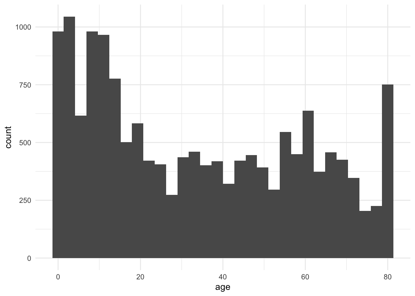
However, the histogram above shows that our sample is skewed towards younger ages. We do, however, see an uptick in frequency around age==80. This is due to the way in which NHANES codes ages; to protect the confidentiality of older subjects, the maximum age that is recorded is 80 (even if the subject’s true age is >80).
full %>%
  ggplot(aes(race)) +
  geom_bar() +
  theme_minimal() +
theme(axis.text.x = element_text(angle = 90, vjust = 0.5, hjust=1)) 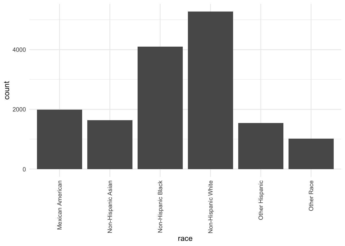
Finally, the above plot shows us the racial composition of our sample. We can see that the majority of subjects identify as Non-Hispanic White and Non-Hispanic Black.
As discussed above, a subject’s food security could possibly serve as an indicator of a socioeconomic stressor. In order for this variable to be meaningful for an analysis, however, we would want our sample to contain individuals at various levels of food security.
Below, we see the distribution of food security in our sample. The individuals in the sample are predominantly food-secure. In order to compare roughly equal sample sizes, if we were to use this variable in an analysis, we might consider converting hh_food_security to a binary secure/not secure variable.
full %>%
  ggplot(aes(hh_food_security)) +
  geom_bar() +
  theme_minimal() +
theme(axis.text.x = element_text(angle = 90, vjust = 0.5, hjust=1)) 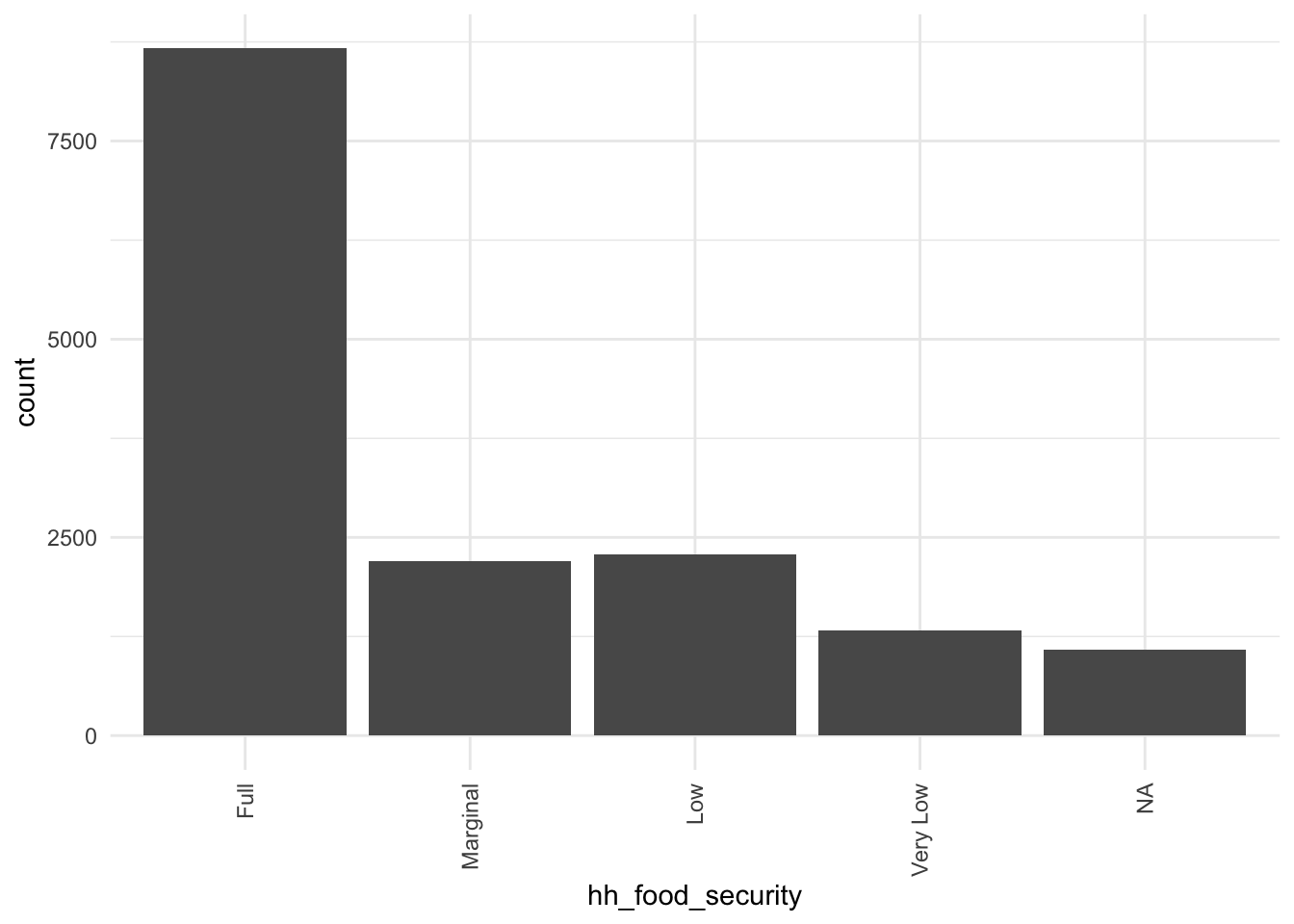
Here, we will examine the distribution of scores from the PHQ depression screener. According to the PHQ, the total score should be interpreted as follows:
full %>%
  ggplot(aes(total_score)) +
  geom_histogram() +
  theme_minimal()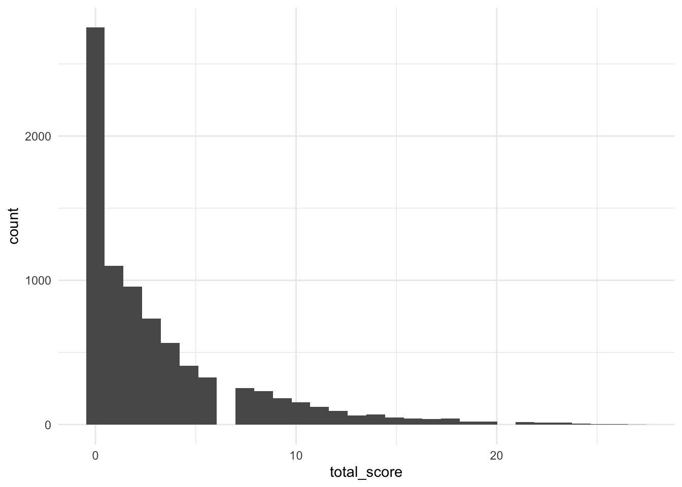
We can see that the vast majority of subjects have a score that is less than 10, indicating minimal or mild depression. Given that there are very few subjects in the sample that reported moderate to severe depression, this variable might not be a very useful predictor for an analysis.
Finally, we can explore the raw distribution of CRP and how CRP varies based on the “stressors” explored above. According to Nehring, Goyal, & Patel (2022), healthy adults will exhibit CRP levels less than or equal to 3 mg/L. CRP levels between 3 and 10 mg/L represent a minor elevation that could be associated with several health conditions, such as obesity, diabetes, smoking, infections, pregnancy, etc. CRP levels between 10 and 100 mg/L could indicate systemic inflammation, such as autoimmune disorders or other inflammatory conditions. CRP levels greater than 100 mg/L could indicate bacterial or viral infections.
Below, we see that the majority of subjects in our sample have very low levels of CRP that are associated with being healthy.
full %>%
  ggplot(aes(crp_mgL)) +
  geom_density()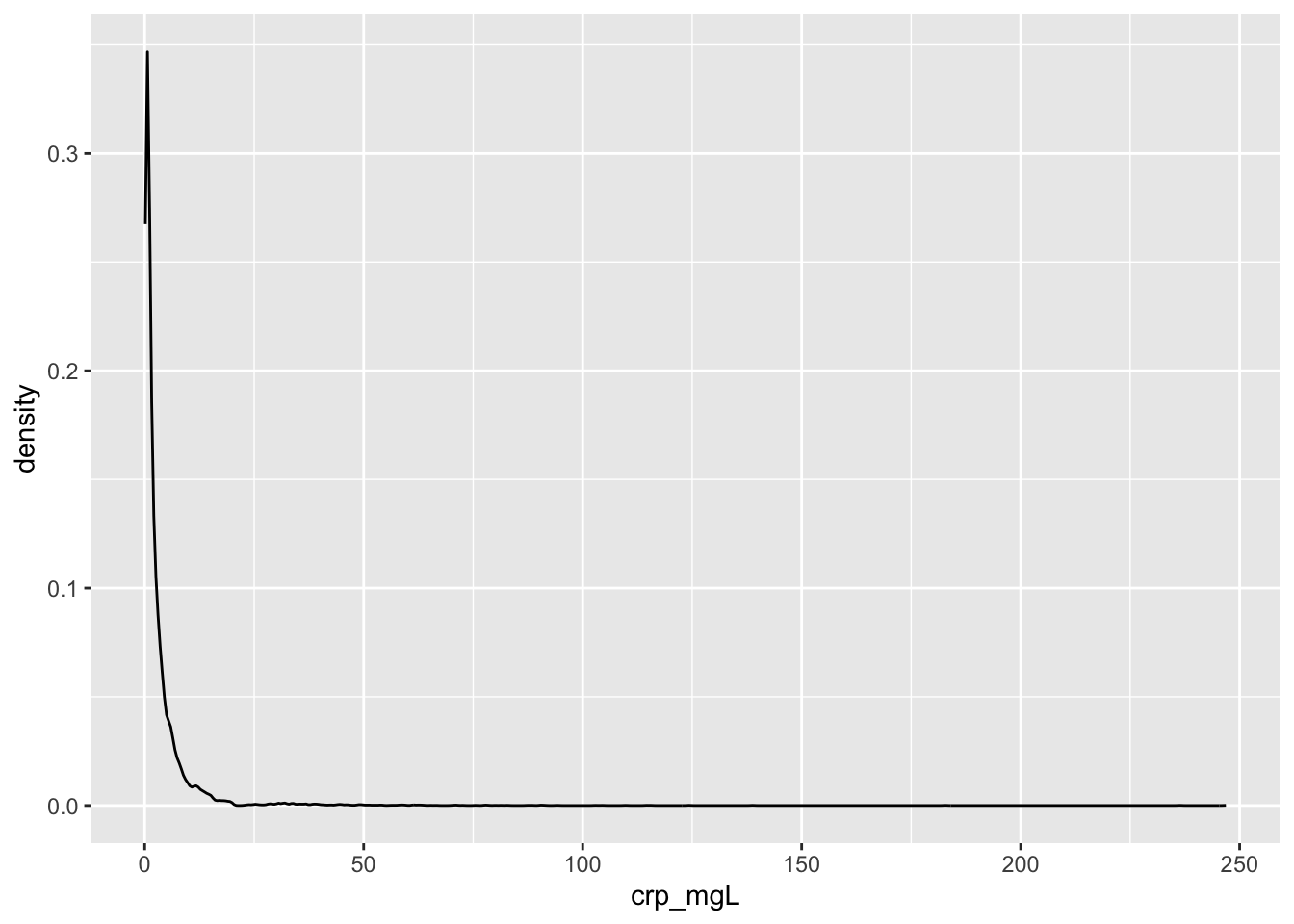
If we look at the CRP levels by food security status, we see that fully food-secure subjects appear to have lower CRP levels than marginal, low, or very low food insecure subjects, but it is unclear if these differences would be significant (especially after controlling for possible confounders).
full %>%
  filter(!is.na(hh_food_security)) %>%
  group_by(hh_food_security) %>%
  summarize(mean_crp = mean(crp_mgL, na.rm=T)) %>%
  ggplot(aes(x=hh_food_security, y = mean_crp)) +
  geom_bar(stat='identity') +
  theme_minimal()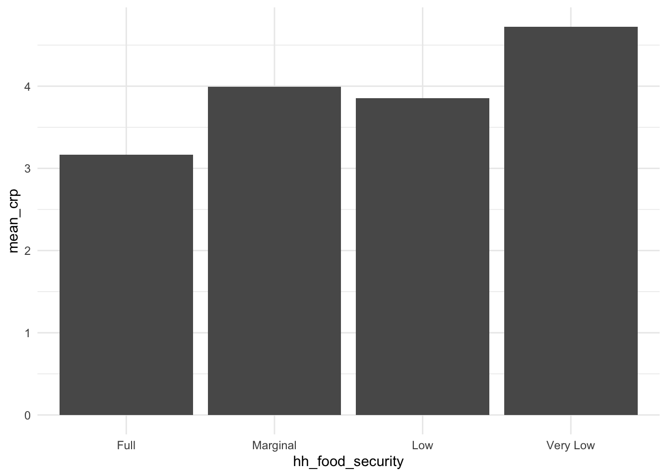
We also see some variation in CRP levels based on depression classification. It could be interesting to see if any of these differences are signifcant.
full %>%
  mutate(
    depression = case_when(
      total_score <= 4 ~ 'Minimal',
      total_score >= 5 & total_score <= 9 ~ 'Mild',
      total_score >= 10 & total_score <= 14 ~ 'Moderate',
      total_score >= 15 & total_score <= 19 ~ 'Moderate-Severe',
      total_score >= 20 ~ 'Severe',
      T ~ NA)
  ) %>%
  filter(!is.na(depression)) %>%
  group_by(depression) %>%
  summarize(mean_crp = mean(crp_mgL, na.rm=T)) %>%
  ggplot(aes(x=depression, y = mean_crp)) +
  geom_bar(stat='identity') +
  theme_minimal()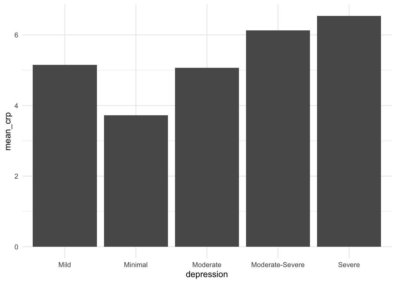
Although I initially envisioned an analysis where both food_security and mental_health could serve as “stressor” variables in an analysis, it could be interesting to do an investigation between food_security and CRP or mental_health and CRP. For both analyses, it would be important to include other predictors that could elevate inflammation, such as weight, diabetes, and other medical conditions.