For this challenge, I will be working with the AB_NYC_2019.csv file.
data <-read_csv(here("posts", "_data", "AB_NYC_2019.csv"))# View datahead(data)
# Use dfSummary!print(summarytools::dfSummary(data,varnumbers=FALSE,plain.ascii=FALSE,style="grid",graph.magnif =0.70,valid.col=FALSE),method="render",table.classes="table-condensed")
Data Frame Summary
data
Dimensions: 48895 x 16
Duplicates: 0
Variable
Stats / Values
Freqs (% of Valid)
Graph
Missing
id [numeric]
Mean (sd) : 19017143 (10983108)
min ≤ med ≤ max:
2539 ≤ 19677284 ≤ 36487245
IQR (CV) : 19680234 (0.6)
48895 distinct values
0 (0.0%)
name [character]
1. Hillside Hotel
2. Home away from home
3. New york Multi-unit build
4. Brooklyn Apartment
5. Loft Suite @ The Box Hous
6. Private Room
7. Artsy Private BR in Fort
8. Private room
9. Beautiful Brooklyn Browns
10. Cozy Brooklyn Apartment
[ 47884 others ]
18
(
0.0%
)
17
(
0.0%
)
16
(
0.0%
)
12
(
0.0%
)
11
(
0.0%
)
11
(
0.0%
)
10
(
0.0%
)
10
(
0.0%
)
8
(
0.0%
)
8
(
0.0%
)
48758
(
99.8%
)
16 (0.0%)
host_id [numeric]
Mean (sd) : 67620011 (78610967)
min ≤ med ≤ max:
2438 ≤ 30793816 ≤ 274321313
IQR (CV) : 99612390 (1.2)
37457 distinct values
0 (0.0%)
host_name [character]
1. Michael
2. David
3. Sonder (NYC)
4. John
5. Alex
6. Blueground
7. Sarah
8. Daniel
9. Jessica
10. Maria
[ 11442 others ]
417
(
0.9%
)
403
(
0.8%
)
327
(
0.7%
)
294
(
0.6%
)
279
(
0.6%
)
232
(
0.5%
)
227
(
0.5%
)
226
(
0.5%
)
205
(
0.4%
)
204
(
0.4%
)
46060
(
94.2%
)
21 (0.0%)
neighbourhood_group [character]
1. Bronx
2. Brooklyn
3. Manhattan
4. Queens
5. Staten Island
1091
(
2.2%
)
20104
(
41.1%
)
21661
(
44.3%
)
5666
(
11.6%
)
373
(
0.8%
)
0 (0.0%)
neighbourhood [character]
1. Williamsburg
2. Bedford-Stuyvesant
3. Harlem
4. Bushwick
5. Upper West Side
6. Hell's Kitchen
7. East Village
8. Upper East Side
9. Crown Heights
10. Midtown
[ 211 others ]
3920
(
8.0%
)
3714
(
7.6%
)
2658
(
5.4%
)
2465
(
5.0%
)
1971
(
4.0%
)
1958
(
4.0%
)
1853
(
3.8%
)
1798
(
3.7%
)
1564
(
3.2%
)
1545
(
3.2%
)
25449
(
52.0%
)
0 (0.0%)
latitude [numeric]
Mean (sd) : 40.7 (0.1)
min ≤ med ≤ max:
40.5 ≤ 40.7 ≤ 40.9
IQR (CV) : 0.1 (0)
19048 distinct values
0 (0.0%)
longitude [numeric]
Mean (sd) : -74 (0)
min ≤ med ≤ max:
-74.2 ≤ -74 ≤ -73.7
IQR (CV) : 0 (0)
14718 distinct values
0 (0.0%)
room_type [character]
1. Entire home/apt
2. Private room
3. Shared room
25409
(
52.0%
)
22326
(
45.7%
)
1160
(
2.4%
)
0 (0.0%)
price [numeric]
Mean (sd) : 152.7 (240.2)
min ≤ med ≤ max:
0 ≤ 106 ≤ 10000
IQR (CV) : 106 (1.6)
674 distinct values
0 (0.0%)
minimum_nights [numeric]
Mean (sd) : 7 (20.5)
min ≤ med ≤ max:
1 ≤ 3 ≤ 1250
IQR (CV) : 4 (2.9)
109 distinct values
0 (0.0%)
number_of_reviews [numeric]
Mean (sd) : 23.3 (44.6)
min ≤ med ≤ max:
0 ≤ 5 ≤ 629
IQR (CV) : 23 (1.9)
394 distinct values
0 (0.0%)
last_review [Date]
min : 2011-03-28
med : 2019-05-19
max : 2019-07-08
range : 8y 3m 10d
1764 distinct values
10052 (20.6%)
reviews_per_month [numeric]
Mean (sd) : 1.4 (1.7)
min ≤ med ≤ max:
0 ≤ 0.7 ≤ 58.5
IQR (CV) : 1.8 (1.2)
937 distinct values
10052 (20.6%)
calculated_host_listings_count [numeric]
Mean (sd) : 7.1 (33)
min ≤ med ≤ max:
1 ≤ 1 ≤ 327
IQR (CV) : 1 (4.6)
47 distinct values
0 (0.0%)
availability_365 [numeric]
Mean (sd) : 112.8 (131.6)
min ≤ med ≤ max:
0 ≤ 45 ≤ 365
IQR (CV) : 227 (1.2)
366 distinct values
0 (0.0%)
Generated by summarytools 1.0.1 (R version 4.3.0) 2023-06-17
# Check for NAsdata %>%summarise(across(everything(), ~sum(is.na(.))))
# Interesting that there are lots of missing data, let's check how many units have no reviewsdata %>%filter(number_of_reviews ==0) %>%nrow()
[1] 10052
Briefly describe the data
This data is probably a collection of all Airbnbs in New York City in 2019, and includes variables such as cost, availability, the neighborhood for where the Airbnb is located, the room type, IDs for both the location and host, and various review information.
Our data seems to already be tidy! Each row represents an Airbnb location, as every location has its own id. Other columns include the place’s name, the host_id for the host of the location, the neighborhood_group and neighborhood the place is located in NYC, the latitude and longitude for the Airbnb, the room_type of the Airbnb, price and minimum_nights that describe the specifics for booking the location, date of last_review, approximate reviews_per_month, the calculated_host_listings_count, and availability_365 for the Airbnb for the year. There are 48,895 rows and 16 columns.
While there are some missing data (such as the name, host_name, last_review, and reviews_per_month). It’s interesting though that the review related columns are both missing 10,052 rows, or 20.26% of all observations. This is probably because these units have never been rented out or are new, so customers have not left any reviews yet. My suspicions are supported because 10,052 rows have number_of_reviews as 0.
# Only column that needs "fixing" is the `room_type`
unique(data$room_type)
# 3 unique values, convert to factorsdata$room_type <-factor(data$room_type)# Convert `last_review` into yearly groupsdata <- data %>%mutate(last_rev_year =year(last_review))
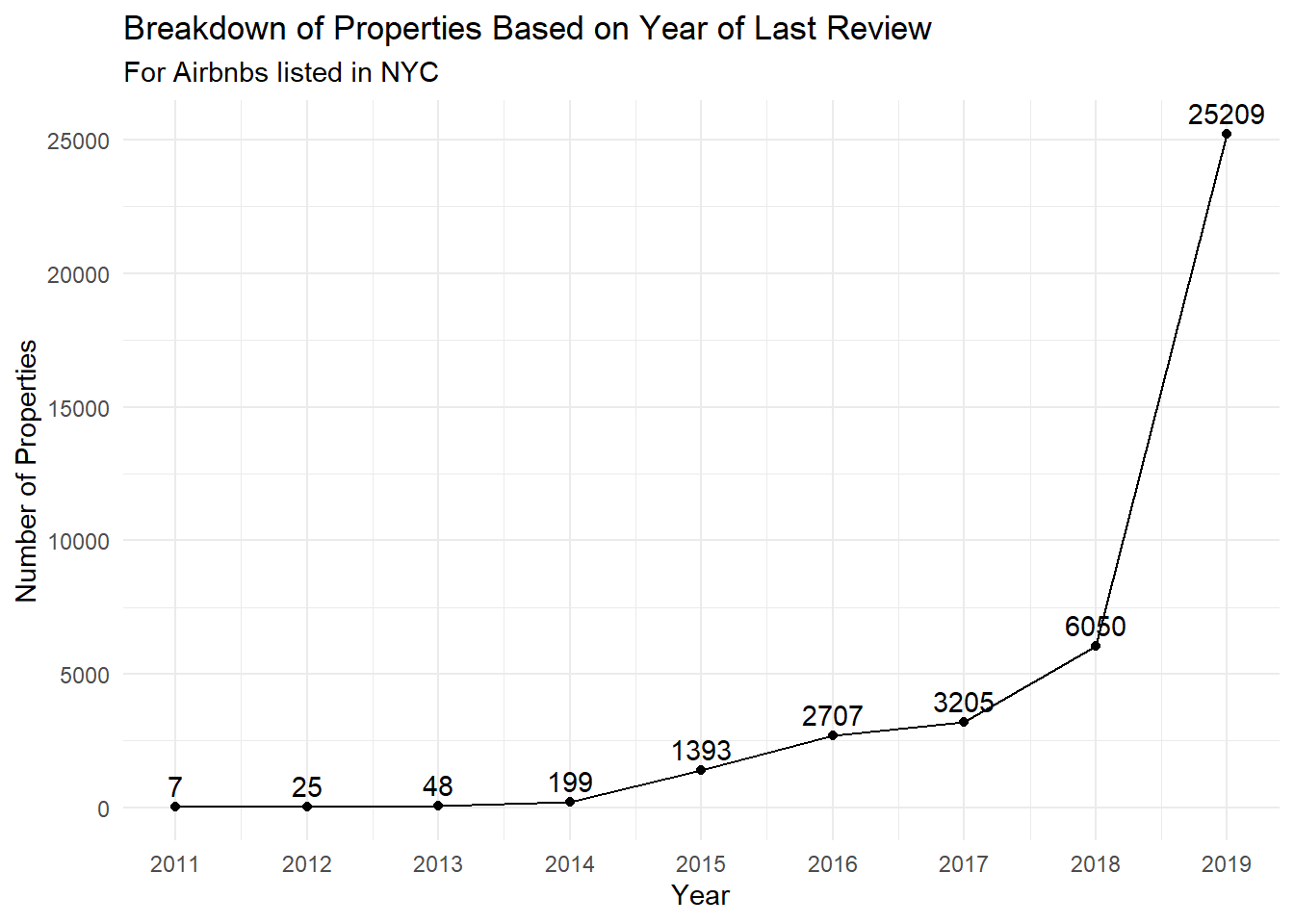
Time Dependent Visualization
For this section, I’ll be looking at the number of properties based on the date of last review, by year. This is because last_review is the only date variable in the dataset. To do this, I will create a time series plot visualizing the dates on the x-axis, and the number of properties on the y-axis. I chose a line graph because this tends to be the best way to visualize time-series related data.
data %>%group_by(last_rev_year) %>%filter(!is.na(last_rev_year)) %>%summarise(num_props =n_distinct(id)) %>%ggplot(aes(x=last_rev_year, y=num_props)) +geom_line() +geom_point() +geom_text(aes(x=last_rev_year, y=num_props, label=num_props), vjust=-0.5) +theme_minimal() +labs(title="Breakdown of Properties Based on Year of Last Review",subtitle="For Airbnbs listed in NYC",x="Year",y="Number of Properties") +scale_x_continuous(breaks=2011:2019, labels=2011:2019)
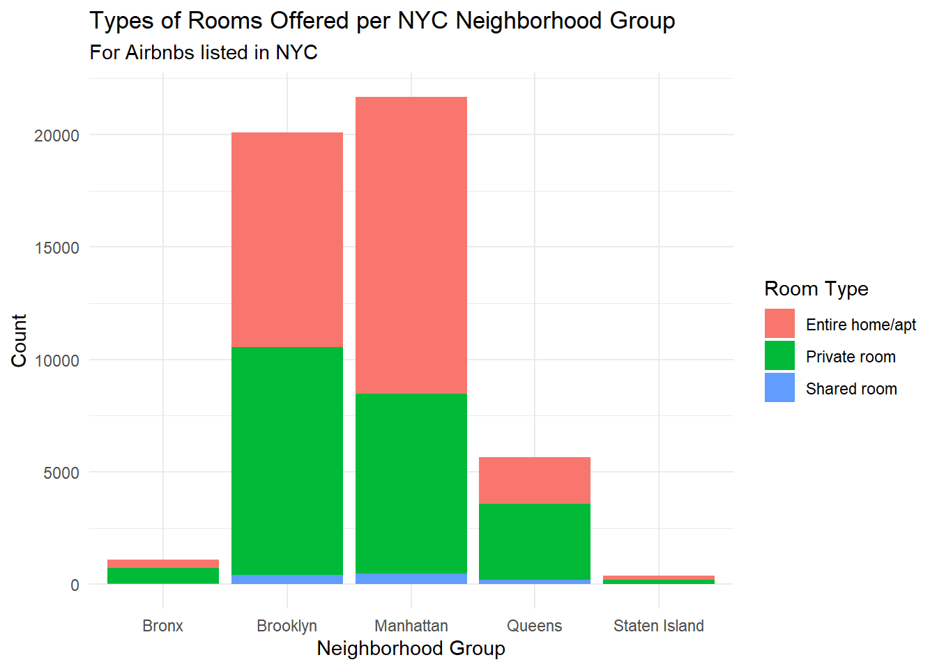
Visualizing Part-Whole Relationships
For this section, I’ll visualize the room_types by each neighborhood_group and use a stacked barchart to visualize this data. This would provide a quick way to compare the number of each room_type across each neighborhood_group.
data %>%group_by(neighbourhood_group, room_type) %>%summarise(val=n_distinct(id)) %>%ggplot(aes(x=neighbourhood_group, y=val, fill=room_type)) +geom_bar(position="stack", stat="identity") +theme_minimal() +labs(title="Types of Rooms Offered per NYC Neighborhood Group",subtitle="For Airbnbs listed in NYC",x="Neighborhood Group",y="Count") +guides(fill=guide_legend(title="Room Type"))
Source Code
---title: "Challenge 6 Solution - Airbnbs in NYC 2019"author: "Linus Jen"description: "Visualizing Time and Relationships"date: "6/20/2023"format: html: toc: true code-copy: true code-tools: true df-print: pagedcategories: - challenge_6 - air_bnb - Linus Jen---```{r}#| label: setup#| warning: false#| message: falselibrary(tidyverse)library(ggplot2)library(here)knitr::opts_chunk$set(echo =TRUE, warning=FALSE, message=FALSE)```## Read in dataFor this challenge, I will be working with the `AB_NYC_2019.csv` file.```{r}data <-read_csv(here("posts", "_data", "AB_NYC_2019.csv"))# View datahead(data)# Use dfSummary!print(summarytools::dfSummary(data,varnumbers=FALSE,plain.ascii=FALSE,style="grid",graph.magnif =0.70,valid.col=FALSE),method="render",table.classes="table-condensed")# Check for NAsdata %>%summarise(across(everything(), ~sum(is.na(.))))# Interesting that there are lots of missing data, let's check how many units have no reviewsdata %>%filter(number_of_reviews ==0) %>%nrow()```### Briefly describe the dataThis data is probably a collection of all Airbnbs in New York City in 2019, and includes variables such as cost, availability, the neighborhood for where the Airbnb is located, the room type, IDs for both the location and host, and various review information.Our data seems to already be tidy! Each row represents an Airbnb location, as every location has its own id. Other columns include the place’s `name`, the `host_id` for the host of the location, the `neighborhood_group` and `neighborhood` the place is located in NYC, the `latitude` and `longitude` for the Airbnb, the `room_type` of the Airbnb, `price` and `minimum_nights` that describe the specifics for booking the location, date of `last_review`, approximate `reviews_per_month`, the `calculated_host_listings_count`, and `availability_365` for the Airbnb for the year. There are 48,895 rows and 16 columns.While there are some missing data (such as the `name`, `host_name`, `last_review`, and `reviews_per_month`). It’s interesting though that the review related columns are both missing 10,052 rows, or 20.26% of all observations. This is probably because these units have never been rented out or are new, so customers have not left any reviews yet. My suspicions are supported because 10,052 rows have `number_of_reviews` as 0.```{r}# Only column that needs "fixing" is the `room_type` unique(data$room_type)# 3 unique values, convert to factorsdata$room_type <-factor(data$room_type)# Convert `last_review` into yearly groupsdata <- data %>%mutate(last_rev_year =year(last_review))```## Time Dependent VisualizationFor this section, I'll be looking at the number of properties based on the date of last review, by year. This is because `last_review` is the only date variable in the dataset. To do this, I will create a time series plot visualizing the dates on the x-axis, and the number of properties on the y-axis. I chose a line graph because this tends to be the best way to visualize time-series related data.```{r}data %>%group_by(last_rev_year) %>%filter(!is.na(last_rev_year)) %>%summarise(num_props =n_distinct(id)) %>%ggplot(aes(x=last_rev_year, y=num_props)) +geom_line() +geom_point() +geom_text(aes(x=last_rev_year, y=num_props, label=num_props), vjust=-0.5) +theme_minimal() +labs(title="Breakdown of Properties Based on Year of Last Review",subtitle="For Airbnbs listed in NYC",x="Year",y="Number of Properties") +scale_x_continuous(breaks=2011:2019, labels=2011:2019)```## Visualizing Part-Whole RelationshipsFor this section, I'll visualize the `room_type`s by each `neighborhood_group` and use a stacked barchart to visualize this data. This would provide a quick way to compare the number of each `room_type` across each `neighborhood_group`.```{r}data %>%group_by(neighbourhood_group, room_type) %>%summarise(val=n_distinct(id)) %>%ggplot(aes(x=neighbourhood_group, y=val, fill=room_type)) +geom_bar(position="stack", stat="identity") +theme_minimal() +labs(title="Types of Rooms Offered per NYC Neighborhood Group",subtitle="For Airbnbs listed in NYC",x="Neighborhood Group",y="Count") +guides(fill=guide_legend(title="Room Type"))```