library(tidyverse)
library(ggplot2)
library(readxl)

knitr::opts_chunk$set(echo = TRUE, warning=FALSE, message=FALSE)Challenge 8 Submission
challenge_8
debt
Joining Data
Read in data
The two data sets I read in were the fed_rate and the debt one.
- fed_rate ⭐⭐⭐
- debt ⭐⭐⭐
# Reading the Fed Data

fed_data <- read_csv("_data/FedFundsRate.csv")

head(fed_data)
# A tibble: 6 × 10
Year Month Day `Federal Funds Target Rate` `Federal Funds Upper Target`
<dbl> <dbl> <dbl> <dbl> <dbl>
1 1954 7 1 NA NA
2 1954 8 1 NA NA
3 1954 9 1 NA NA
4 1954 10 1 NA NA
5 1954 11 1 NA NA
6 1954 12 1 NA NA
# ℹ 5 more variables: `Federal Funds Lower Target` <dbl>,
# `Effective Federal Funds Rate` <dbl>, `Real GDP (Percent Change)` <dbl>,
# `Unemployment Rate` <dbl>, `Inflation Rate` <dbl># Reading the Debt Data
debt_data <- read_excel("_data/debt_in_trillions.xlsx")
head(debt_data)# A tibble: 6 × 8
`Year and Quarter` Mortgage `HE Revolving` `Auto Loan` `Credit Card`
<chr> <dbl> <dbl> <dbl> <dbl>
1 03:Q1 4.94 0.242 0.641 0.688
2 03:Q2 5.08 0.26 0.622 0.693
3 03:Q3 5.18 0.269 0.684 0.693
4 03:Q4 5.66 0.302 0.704 0.698
5 04:Q1 5.84 0.328 0.72 0.695
6 04:Q2 5.97 0.367 0.743 0.697
# ℹ 3 more variables: `Student Loan` <dbl>, Other <dbl>, Total <dbl>Briefly describe the data
Fed Rate: This data contains basic information about the federal economy. It includes measurements around the Fed Rate, GDP, Inflation, Unemployment, and other economical measures.
Debt Rate: This data contains measurements of various types of debt.
Tidy Data (as needed)
For the Fed Data, from quick observation there is no data that needs to be tidied, except for reformatting the Year, Month, and Day into a Data Column.
# Creating the date column for the fed rate
date_col <- paste(fed_data$Year, fed_data$Month, fed_data$Day)

fed_data <- fed_data %>%
  mutate(Date = as.Date(date_col,format = "%Y %m %d"), .before=`Year`)

fed_data <- fed_data[-c(2, 3, 4)]

head(fed_data)
# A tibble: 6 × 8
Date `Federal Funds Target Rate` `Federal Funds Upper Target`
<date> <dbl> <dbl>
1 1954-07-01 NA NA
2 1954-08-01 NA NA
3 1954-09-01 NA NA
4 1954-10-01 NA NA
5 1954-11-01 NA NA
6 1954-12-01 NA NA
# ℹ 5 more variables: `Federal Funds Lower Target` <dbl>,
# `Effective Federal Funds Rate` <dbl>, `Real GDP (Percent Change)` <dbl>,
# `Unemployment Rate` <dbl>, `Inflation Rate` <dbl>Similarly, for the Debt Data we had to create a Date variable as well, which consisted of expaning the year to be four digits, and formatting the quarter to be the first of each corresponding month. (Q1=March, Q2=June, Q3=September, Q4=December).
# Creating the date column for the debt table

debt_data[c('Year','Month')] <- str_split_fixed(debt_data$`Year and Quarter`, ':', 2)
debt_data <- debt_data[,c(9,10,1:8)]

# Changing the year to match
debt_data <- mutate(debt_data, 'Year'=paste('20',debt_data$Year, sep=''))
# Changing the month to match
debt_data$Month[debt_data$Month == 'Q1'] <- '3'
debt_data$Month[debt_data$Month == 'Q2'] <- '6'
debt_data$Month[debt_data$Month == 'Q3'] <- '9'
debt_data$Month[debt_data$Month == 'Q4'] <- '12'
# Adding in a day
debt_data <- debt_data %>% mutate(Day = 1, .after=Month)

# Formatting into Date
date_col <- paste(debt_data$Year, debt_data$Month, debt_data$Day)

debt_data <- debt_data %>%
  mutate(Date = as.Date(date_col,format = "%Y %m %d"), .before=`Year`)

debt_data <- debt_data[-c(2, 3, 4, 5)]

head(debt_data)
# A tibble: 6 × 8
Date Mortgage `HE Revolving` `Auto Loan` `Credit Card` `Student Loan`
<date> <dbl> <dbl> <dbl> <dbl> <dbl>
1 2003-03-01 4.94 0.242 0.641 0.688 0.241
2 2003-06-01 5.08 0.26 0.622 0.693 0.243
3 2003-09-01 5.18 0.269 0.684 0.693 0.249
4 2003-12-01 5.66 0.302 0.704 0.698 0.253
5 2004-03-01 5.84 0.328 0.72 0.695 0.260
6 2004-06-01 5.97 0.367 0.743 0.697 0.263
# ℹ 2 more variables: Other <dbl>, Total <dbl>Join Data
My methodology in joining is combining the debt data of each quarter with the various measurements we are given in Fed Rates on those given months. For example, Q1 corresponding with March, Q2 corresponds with June, Q3 corresponds with September and Q4 corresponds with December. So as we can see in my data mutation, I expanded the years to be four digits and separated the quarter from the year in the Debt data so we could join the two.
I only wanted to have entries where we had both the Debt and Fed Data, so I chose to do a right join, since there were a lot less entries in the Debt Data.
combined_data <- fed_data %>% right_join(debt_data, by = join_by(Date))

head(combined_data)
# A tibble: 6 × 15
Date `Federal Funds Target Rate` `Federal Funds Upper Target`
<date> <dbl> <dbl>
1 2003-03-01 1.25 NA
2 2003-06-01 1.25 NA
3 2003-09-01 1 NA
4 2003-12-01 1 NA
5 2004-03-01 1 NA
6 2004-06-01 1 NA
# ℹ 12 more variables: `Federal Funds Lower Target` <dbl>,
# `Effective Federal Funds Rate` <dbl>, `Real GDP (Percent Change)` <dbl>,
# `Unemployment Rate` <dbl>, `Inflation Rate` <dbl>, Mortgage <dbl>,
# `HE Revolving` <dbl>, `Auto Loan` <dbl>, `Credit Card` <dbl>,
# `Student Loan` <dbl>, Other <dbl>, Total <dbl>A simple observation we could make is by comparing two different rates. We can do this by graphing the two and making comparisons about the lines.
combined_data %>%
  ggplot(aes(Date)) +
  geom_line(aes(y = combined_data$Total, color='Red')) +
  geom_line(aes(y = combined_data$`Inflation Rate`, color='Blue')) +
  ylab("Inflation Rate/Debt")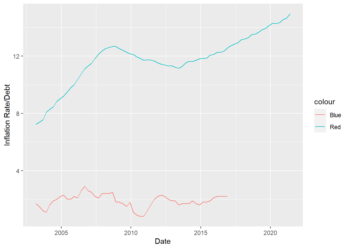
If we look closely we can see something interesting. We can see that when the inflation rate changes, there is a bit of a lag in the Debt graph, for example right when the inflation rate drops in 2010, the debt graph takes 3ish years to bottom out as well. The same observation can be made for when the inflation rate spikes around 2006.