The data set that I chose pertains to salary data for various careers, education levels, gender, and experience. I am interested in investigating this data, as it would allow people to see how their salary compares to people with similar age, job titles, education and experience level.
Looking into the authors’ process to gathering this data, they do not provide much. They state that this data is gathered from surveys, job posting sites, and “other publicly available sources”. These sources can come with uncertainty as people could lie on surveys as they could be uncomfortable with sharing their real salary. We also do not know what is included in “publicly available sources”. But assuming that these sources are trust worthy, pairing this with job posting sites can be very useful in creating numerous data points.
Another area this source is lacking is the type of companies they are sampling from, again another assumption is that they are surveying people from various companies and the data from job posting websites contains multiple employers/types of employers so we have a breadth of data. Even though we don’t know which companies this data comes from we can note that this is primarily professionals working in industry, with an emphasis on software, data science, and similar fields.
When looking into what region this data came from, I could not find anything. So, I looked and compared this to the salaries of similar jobs with similar experience in the United States, and they were similar. With that, I believe that although this may not be perfect, it is certainly sufficient for someone to use this data in the US to compare their salary to.
Code
workers_tidy <-read_csv("_data/Salary_Data.csv")
Rows: 6704 Columns: 6
── Column specification ────────────────────────────────────────────────────────
Delimiter: ","
chr (3): Gender, Education Level, Job Title
dbl (3): Age, Years of Experience, Salary

ℹ Use `spec()` to retrieve the full column specification for this data.
ℹ Specify the column types or set `show_col_types = FALSE` to quiet this message.
Code
workers_tidy
Cleaning the Data Set
Originally, I did not find anything wrong with the data in terms of tidying it up or formatting it. But when doing further analysis I found that some entries in Education Level were recorded as ‘phD’ instead of ‘PhD’, so I went ahead and fixed that. In addition to this, Bachelor’s Degree was listed as both “Bachelor’s” and “Bachelor’s Degree”, so I combined them to “Bachelor’s”. Master’s Degree was also split like this as well and the same changes were made
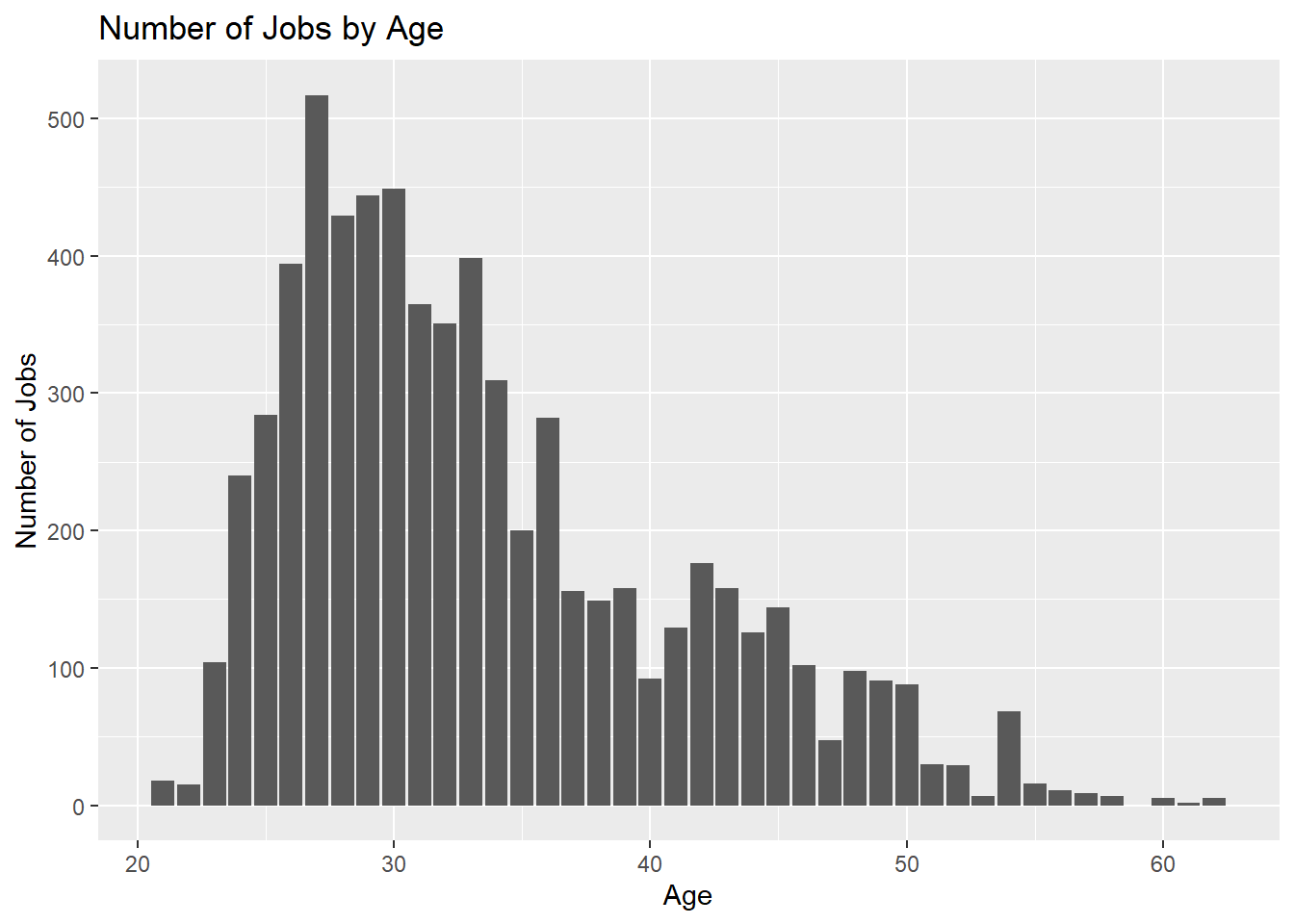
# Adding age distribution table# Putting it into bar chart form as wellggplot(data=subset(workers_tidy, !is.na(Age)), aes(x=Age)) +geom_bar() +labs(y="Number of Jobs", x ="Age") +ggtitle("Number of Jobs by Age")
The first variable is Age, which is simply the age of the employee, this variable is quite self explanatory so I will leave it at that. From above we can see the minimum age is 21, and the maximum age is 62. Below the table of calculated data, we have a plot that allows the viewing of the complete distribution. It can be noted that either this sample contains more jobs for younger professionals, or there are more jobs available for younger professionals.
Code
max_exp <-max(workers_tidy$`Years of Experience`, na.rm=TRUE)min_exp <-min(workers_tidy$`Years of Experience`, na.rm=TRUE)mean_exp <-mean(workers_tidy$`Years of Experience`, na.rm=TRUE)age_table <-matrix(c(min_exp, max_exp, max_exp-min_exp, mean_exp), ncol=4, byrow=TRUE)colnames(age_table) <-c('Min', 'Max', 'Range', 'Mean')rownames(age_table) <-c('Years of Experience')age_table
                    Min Max Range     Mean
Years of Experience   0  34    34 8.094687
Code
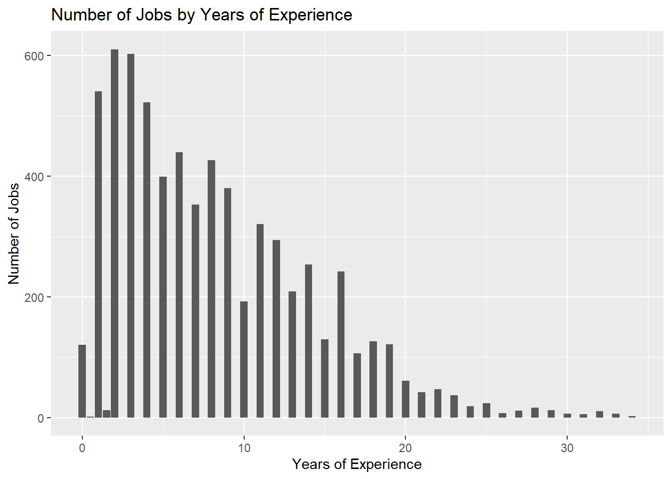
# Putting it into bar chart form as wellggplot(data=subset(workers_tidy, !is.na(`Years of Experience`)), aes(x=`Years of Experience`)) +geom_bar() +labs(y="Number of Jobs", x ="Years of Experience") +ggtitle("Number of Jobs by Years of Experience")
Second, we have Experience Level, which is pretty similar to age, just that this is the number of years someone has been working. By simple analysis we can see that the average is around 8 years. In addition we can see similar statistics that we represented with age. The graph also shows us that we are very heavily sampled from jobs that are in the beginning of one’s career.
Code
table(workers_tidy$`Gender`)
Female   Male  Other
  3014   3674     14
Code
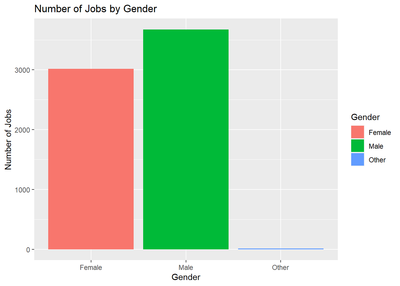
# Putting it into bar chart form as wellggplot(data=subset(workers_tidy, !is.na(Gender)), aes(x=Gender,fill=Gender)) +geom_bar() +labs(y="Number of Jobs", x ="Gender") +ggtitle("Number of Jobs by Gender")
Next, Gender is split into three categories: Male, Female, or Other. Above we can see the exact count for both, with it coming out to be around 54% for males, and 45% for females and 0.2% for Other. To see the distribution a bar chart has been provided.
Code
table(workers_tidy$`Education Level`)
 Bachelor's High School    Master's         PhD
       3023         448        1861        1369
Code
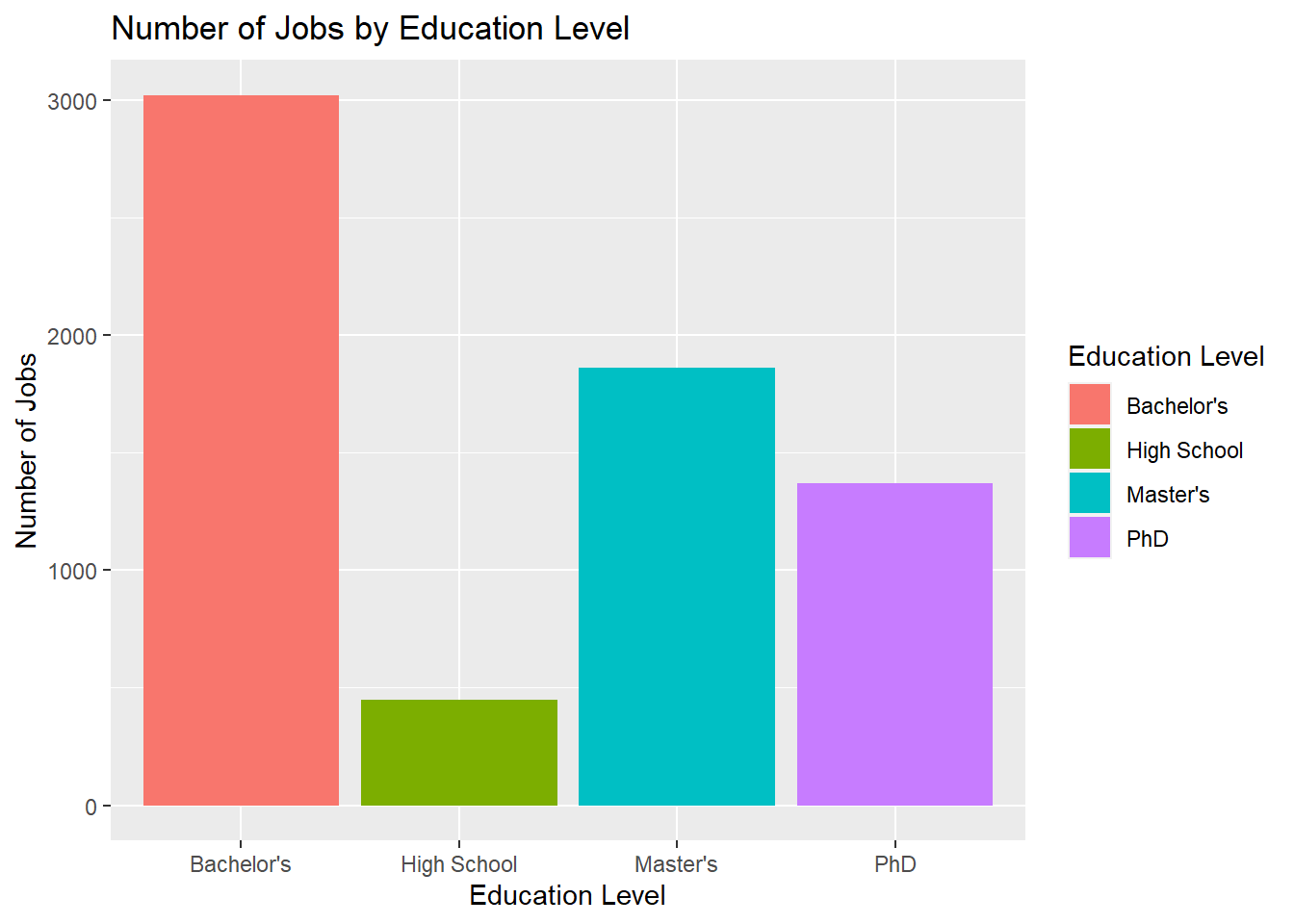
# Put this into bar plot instead# Putting it into bar chart form as wellggplot(data=subset(workers_tidy, !is.na(`Education Level`)), aes(x=`Education Level`,fill=`Education Level`)) +geom_bar() +labs(y="Number of Jobs", x ="Education Level") +ggtitle("Number of Jobs by Education Level")
Education Level is spread out between High School Diploma, Bachelor’s, Master’s and PhD. Similarly we can see that distribution above. This data has been provided in both tabular and graph form. As we’d expect with industry jobs, there is low demand for people with only a HS Diploma and a larger market for those with a Bachelor’s.
# Putting it into bar chart form as wellggplot(data=subset(title_count, Freq >75), aes(x=Var1,y=Freq,fill=Var1)) +geom_bar(stat='identity') +labs(y="Number of Jobs", x ="") +ggtitle("Number of Jobs by Title (More than 50)") +theme(axis.text.x =element_text(angle =45, vjust=1, hjust =1))
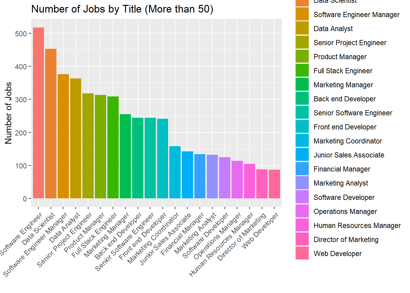
The final variable Job Title is where we can start to see more variance. From the above command, we see that there are around 194 different jobs represented out of the 6700 total samples. From the analysis above, we can see that Software Engineer, Data Scientist, Software Engineer Manager, Data Analyst, Senior Project Engineer, and Product Engineer are the six most popular jobs in the data set.
In addition to listing the 6 most popular jobs, we graph all jobs where they occur more than 75 times. We cut it off at 75 just so the graph was readable. It is very interesting to see many of these titles have to do with engineering, computer science, or data analytics.
Research Questions
This data has plenty to offer in terms of analysis. I want to focus on how Age and Experience affect the salary of an individual. First, I will look into the entire data set of all professions. Then I will look into how this compares to jobs in my field (Computer Science, Data Science, etc.).
After analyzing the question listed above, I wanted to look deeper into the industry I am interested in and how roles/fields affect salaries with respect to age. I was curious on how the roles/fields were distributed and if there were certain niches for each or if some were outliers compared to other counterparts.
General Analysis
As aforementioned, the first two plots will showcase any correlation between Age and Salary, and Years of Experience and Salary. From my general understanding of salaries, I predict that there will be a positive correlation between both of these variables and salaries, but I will be curious to see if there are any points in one’s career that this plateaus.
Code
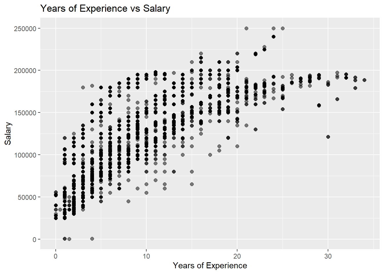
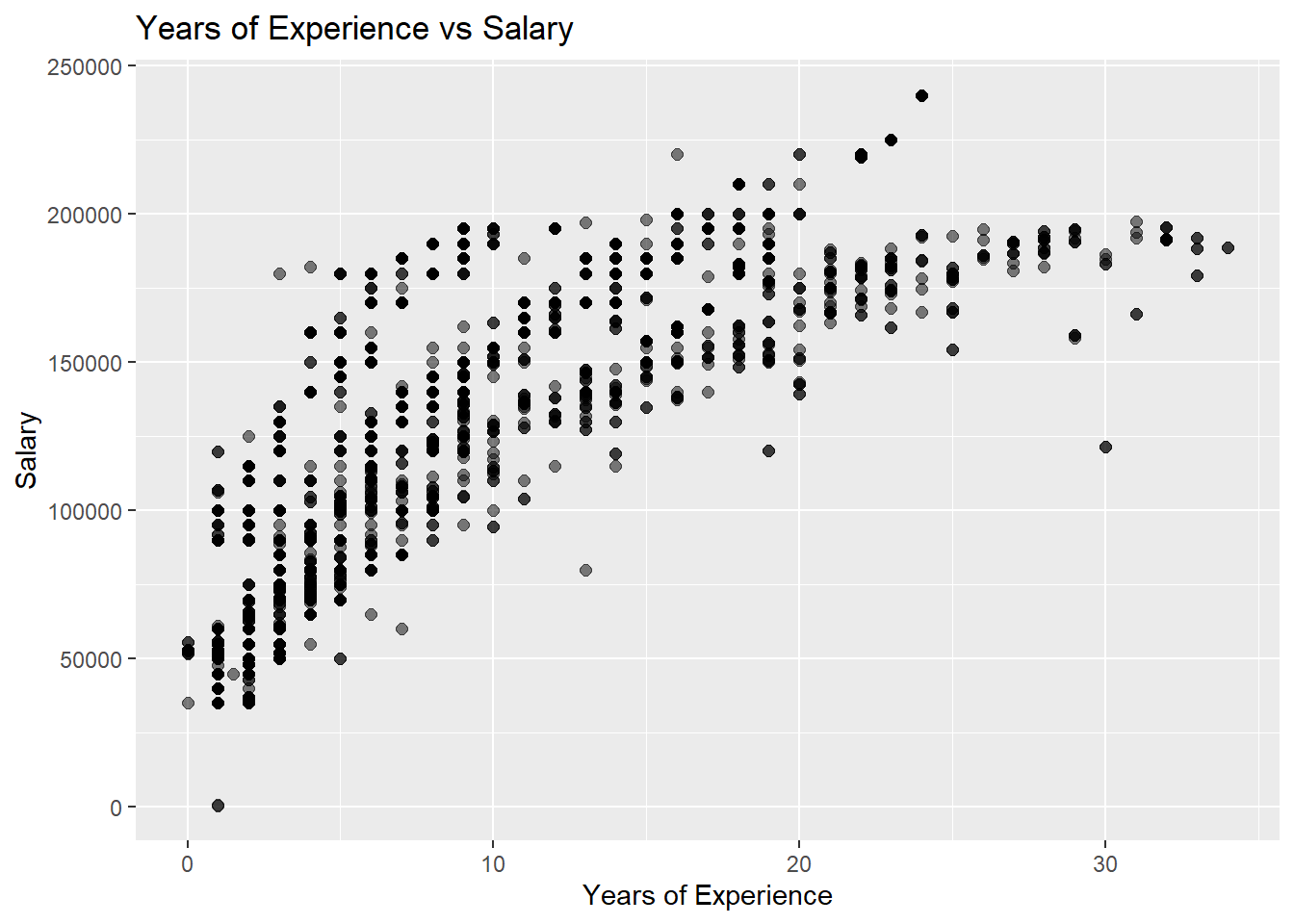
ggplot(subset(workers_tidy, !is.na(`Years of Experience`)), aes(x=`Years of Experience`, y=`Salary`)) +geom_point(size=2, alpha=0.5) +ggtitle("Years of Experience vs Salary")
From the plot above, we can see some very interesting points. If we focus on zero to twenty years of experience we see a fairly steady growth of salary. Another interesting point about this section is that there are a large range of salaries for people with the same years of experience, the difference is that the majority of salaries are increasing in this area.
Also, we are able to see that around these trends there is a heavier density of points. This shows that the trend line is not only an average, but also very common among the data points.
Code
count_years <-as.data.frame(table(workers_tidy$`Years of Experience`))count_years$Var1 <-as.numeric(as.character(count_years$Var1))total <-sum(count_years[which(count_years$Var1 >20),2])
Looking on from twenty years of experience and onward, we notice the curve flattening out. I believe that this is due to multiple factors. The first is that people are not job switching as much, so there is less competition between companies to pay employees better. People are not job hopping as frequently in this age range because they more than likely have a family or are committed to living in a specific area. Another factor may be that companies are only willing to offer so much to one individual, such as a salary cap for people in certain positions.
Also, there may not have been enough data gathered on this particular group. From the small snippet above, we can see only 244 entries are for this particular age group. If these jobs were sampled from a similar company/demographic that may be the reason we see such similarities in the data.
Code
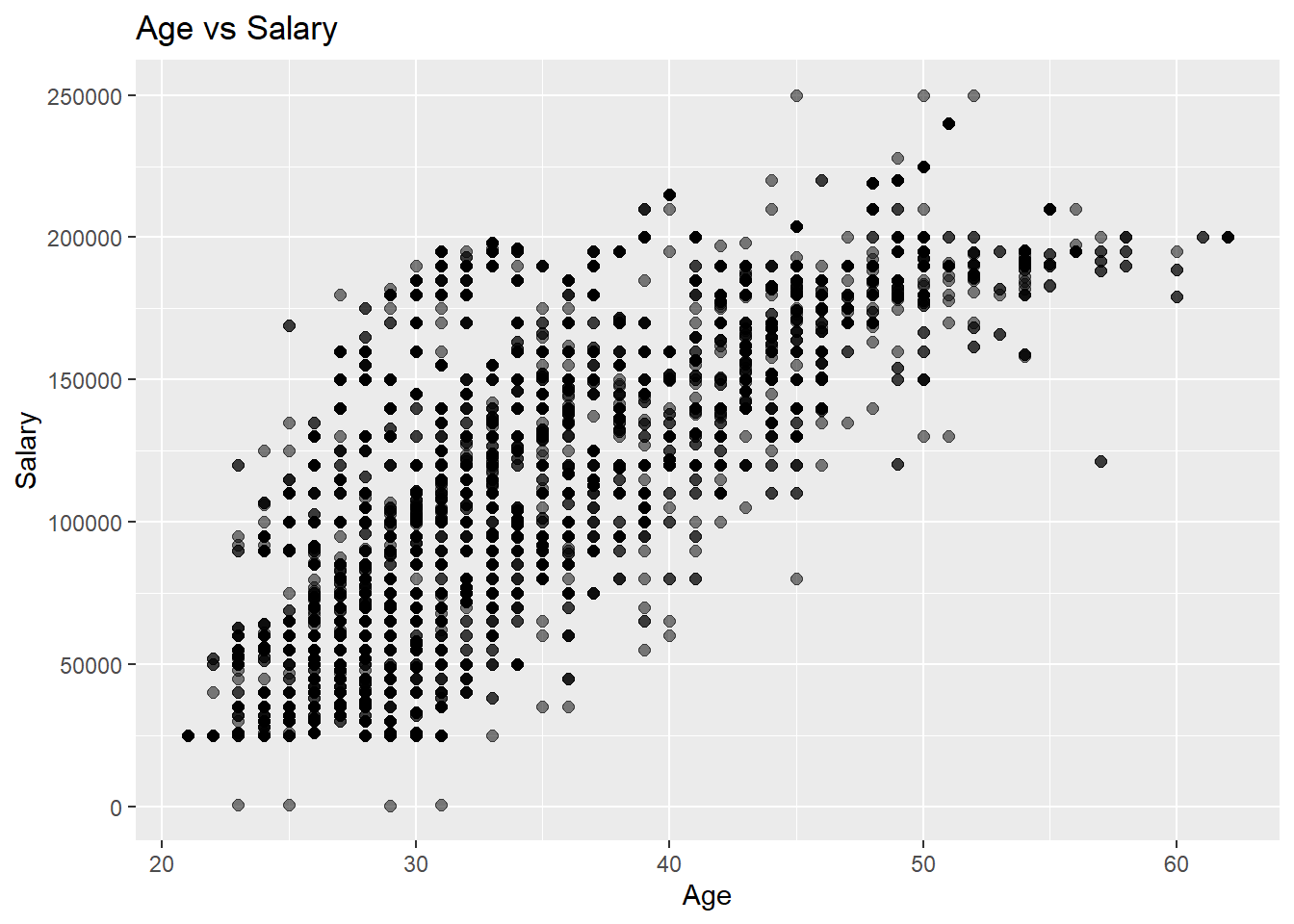
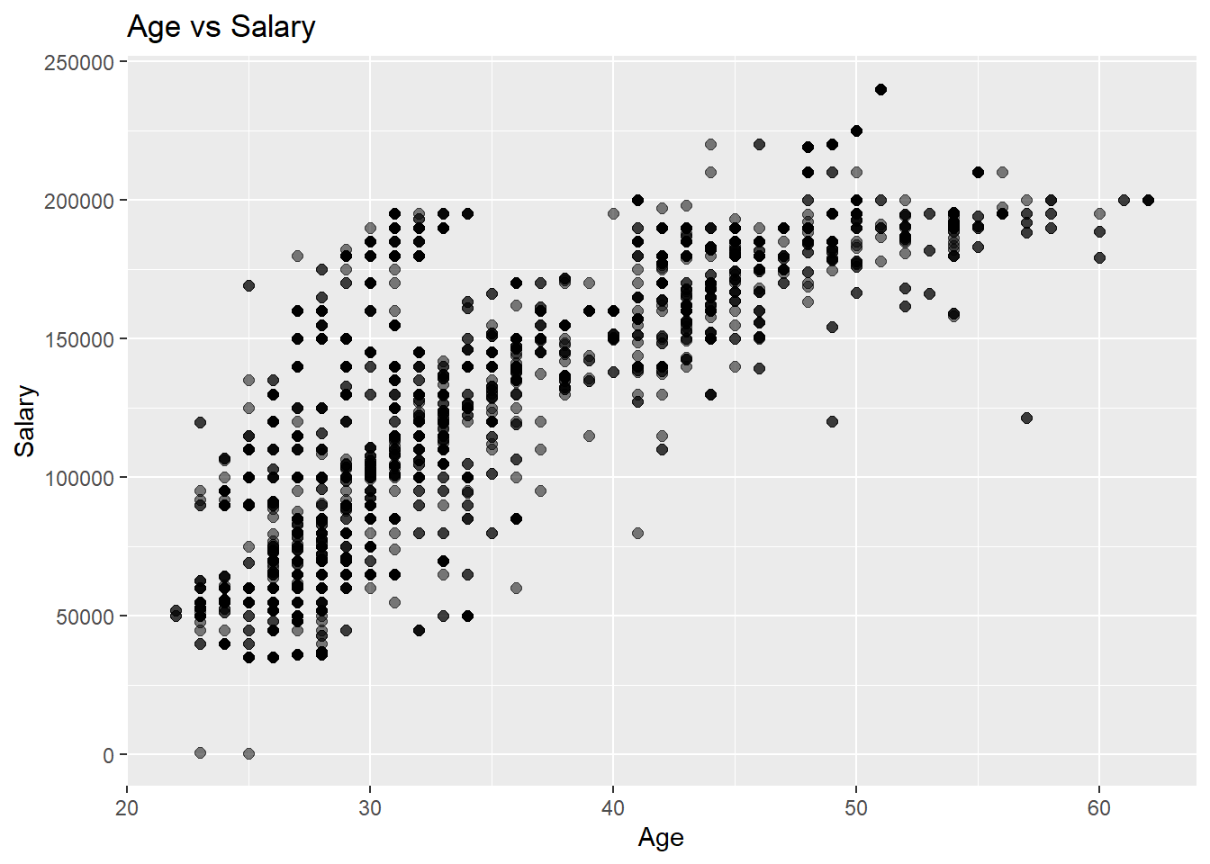
workers_tidy %>%ggplot(aes(x=`Age`, y=`Salary`)) +geom_point(size=2, alpha=0.5) +ggtitle("Age vs Salary")
In this data we can see a very similar plot as the Years of Experience versus Salary plot. One key difference is that this one seems to plateau around 52 years of age which seems to be a bit later in the distribution than the plateau of the experience plot.
An interesting note about this plot is that the points seem to be evenly distributed for the range of salaries. Unlike the experience graph where we saw a dark band through the center, this one seems a bit more spread out.
Similarly to the previous plot there are a lot less samples around where this plateau takes place. But there is even a smaller portion of samples for workers over 50. I think this is due to the fact that people are close to retiring and that people are getting promoted less and less as they approach this age. In my experience young professionals are able to make higher increases in pay more quickly the earlier they are in their career, then as they get older, these promotions are harder to come by.
The final thing to note about age and experience for these two plots is that they are heavily correlated. The one factor that may shift these distributions is degree level. Which we will look at in the next plot.
Code
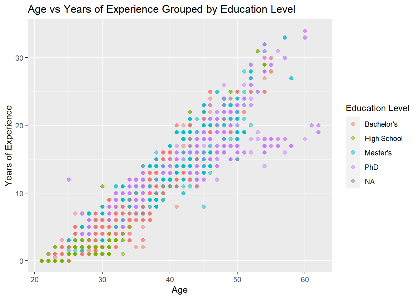
workers_tidy %>%ggplot(aes(x=`Age`, y=`Years of Experience`, color=`Education Level`)) +geom_point(size=2, alpha=0.5) +ggtitle("Age vs Years of Experience Grouped by Education Level")
This plot is extremely interesting as it shows just how much the two are coordinated. We can see that all degree levels follow the trend very closely, except PhD which has a weird branch with around 17 years of experience.
Industry Specific Analysis
Now, I want to focus on jobs that pertain to my career. I looked through all the jobs and picked out key words that were related to my career path. Below I have listed all of these. In the following code block, we mark all of these jobs with “Industry” or “Not”, denoting whether they fall in the given industry.
Key words are: - Software - Engineer - Developer - Data
In the code above, we simply put a marker on whether a job was in the given industry or not.
Below we will recreate both graphs above. Starting with years of experience.
Code
ggplot(subset(workers_tidy, marked=='Industry'),aes(x=`Years of Experience`, y=`Salary`)) +geom_point(size=2, alpha=0.5) +ggtitle("Years of Experience vs Salary")
Comparing this graph to the complete data set graph on comparing salary to years of experience, we can see that there salary from 0-20 years of experience is slightly higher for my field, but about the same from onward. Below is a graph overlaying both of these plots.
Code
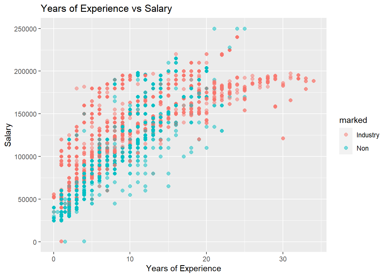
workers_tidy %>%ggplot(aes(x=`Years of Experience`, y=`Salary`, color=marked)) +geom_point(size=2, alpha=0.5) +ggtitle("Years of Experience vs Salary")
Above, in Red we have only the jobs that are in the disciplines I am interested in. In Blue, we have all jobs (including the ones in blue).
This plot further confirms that the salary in my field is slightly higher than average, but this seems to be only up until about 15 years of experience. Then it starts to get very close as the salaries plateau. I would like to see more non-industry data for 20 years of experience and up as there is not much provided in this plot.
Next, we will look at comparing the age of people in the field I’m interested in and their salaries compared to the complete distribution.
First, we will look at the specific field first, so we can get a good understanding of what we’re looking at before we compare.
Code
ggplot(subset(workers_tidy, marked=='Industry'),aes(x=`Age`, y=`Salary`)) +geom_point(size=2, alpha=0.5) +ggtitle("Age vs Salary")
In this plot, we have a very interesting curve. It seems that throughout one’s career in the given fields, the salaries increase, then plateau, and repeat this behavior a few times. My hypothesis for this behavior is that many of the careers in these fields follow the same behavior. This behavior is a promotion every few years, then another promotion after a similar period. If these jobs were sampled from the same company or ones that operate in a similar manner, this would explain the deterministic behavior in the plot.
Now, we will compare these jobs to all the sampled jobs, this plot can be seen below.
Code
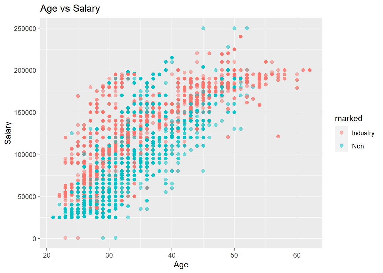
workers_tidy %>%ggplot(aes(x=`Age`, y=`Salary`, color=marked)) +geom_point(size=2, alpha=0.5) +ggtitle("Age vs Salary")
In this plot, the colors represent the same distributions from the previous combined plot. This one is a bit more telling than the experience plot. Here we can see up to around 50 years of age that jobs in the industry dominate non-industry jobs. I say that this is more telling because we have a lot more data for non-industry jobs for a larger period so we have a larger sample to compare to making these conclusions more significant.
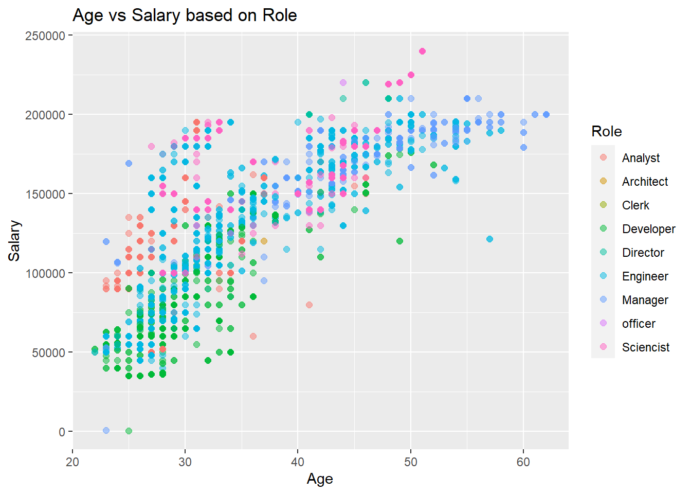
The final piece of analysis we’re going to look at is how the title within the industries I’m interested affects salary. We are going to do this in two separate ways. The first is dividing them based on role, i.e. Developer, Officer, Analyst, Director, etc. and the other is going to be based off of field, i.e. data, software, engineering, etc.
In this plot we can see that Developer, Engineer, Director and Manager all dominate the plot in terms of quantity. But, what is also interesting and self explanatory is that most of the higher paying roles are Managerial Roles, where the lower paying jobs are developers. One job that follows the positive trend and seems to be evenly distributed is an engineer. It seems that this position is valued through ones career.
Another trend we can see is that Developers are paid less than their counterparts in other rolls. As aforementioned there are many developer jobs, but they seem to be more common for younger individuals, with the salaries being lower than other jobs such as Engineers, Analysts and Scientists.
Code
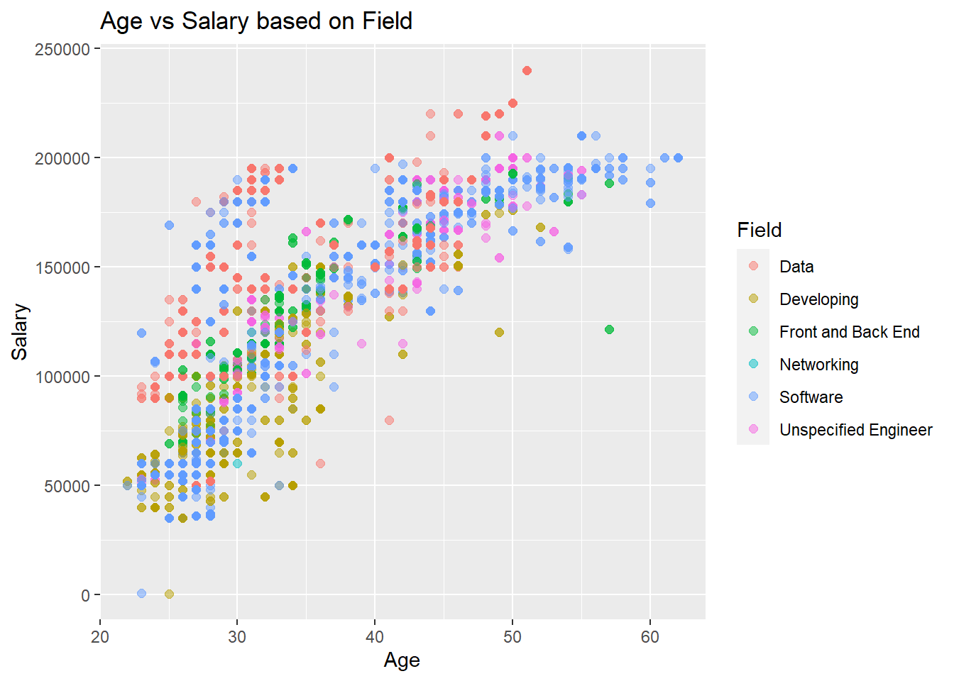
mark_field <-function(entry) { job <-tolower(entry)if (grepl("data",tolower(job))) {return('Data') } elseif (grepl("software",tolower(job))){return('Software') } elseif (grepl("network",tolower(job))){return('Networking') } elseif (grepl("full stack",tolower(job))){return('Front and Back End') } elseif (grepl("developer",tolower(job))){return('Developing') } elseif (grepl("engineer",tolower(job))){return('Unspecified Engineer') } else {return('Not Found') }}industry_jobs <-subset(workers_tidy, workers_tidy$marked =="Industry")industry_jobs$Field <-map_chr(industry_jobs$`Job Title`, mark_field)ggplot(industry_jobs,aes(x=`Age`, y=`Salary`, color=Field)) +geom_point(size=2, alpha=0.5) +ggtitle("Age vs Salary based on Field")
This plot has a very similar look in color distributions as the previous graph. This is self-explanatory as roles and fields somewhat over lap. In the division of this data, I tried to label the most specific fields first, such as Data and Software, and then if a job title did not fit into there I used more general fields such as Developing, Engineering, and others.
Looking closely, we can see that there is a noticeable difference between general developing and Front and Back End developing. This may be due to the fact the latter requires a more specific skill set which is more desirable and competitive with pay.
We can also see that jobs with data dominate in salary for years 20-35, but then the salaries fall back into normal range. This could possibly be due to the fact that data is a competitive/popular field coming out of college so industry professionals want to hire the best possible candidates.
Similar to the previous plot, we see that the software field follows the positive trend very closely and has a wide range of salaries but most fall into a similar range. This can be because software is a very common field to go around so the market may have settled and found a stable price point for age and salary.
Conclusions
In this data I have looked at not only how age and experience affect most jobs but also how it affects jobs in the industries I’m interested in and how the salaries compare between the two. From this analysis on the two variables (age and experience) and their affect on salary for given jobs, I have found interesting trends, and confirmed previous thoughts. In addition to these confirmations, I have also found out how the field and role within the industries I’m interested affect affects the salary and what the projections look like across those different careers.
Even though I was able to discover new things and confirm old ideas, there is still plenty left on the table that I was not able to discover because of limitations from the data set.
What I’ve Learned
My previous thoughts were that age and experience positively correlate with salary, which is true. My second was that people in the industry I am hoping to enter (engineering, data, computer science) would make slightly more than jobs not in this field. This was also confirmed in the plots where we compared industry salaries (in red) to non-industry salaries (in blue) versus both age and experience.
Going even deeper into each of these plots you notice small trends. For example, in both age and experience for the total distribution you see the trend of salaries plateauing after a certain age/number of years. I listed many possible reasons for this, but it would be interesting to see if the companies that provided these numbers would elaborate on why these trends are present.
The other trend that I found very interesting, was that of the Age vs Salary plot for only industry jobs. If one looks closely to the darker regions of the graph, there is a staircase like behavior to it. I noted that this could be due to the progression of ones career with promotions. This would explain why jobs from various companies have similar paths, as careers across various companies as they have various levels of jobs and one progresses through these ranks throughout their career.
Finally, I’ve learned how the role/field within my industry can influence job choices and even what path I go to as I gain more experience. For example, I see that the demand for certain roles diminishes as a career progresses. It seems that jobs in data have a high entry point, but as one’s career progresses it seems that it plateaus. Where as it seems that software has a slightly lower entering salary, but there is constant growth.
Assuming one is obtaining a degree in a related field and finds the work entertaining they can use this data to look for specific roles and fields to maximize their salary capabilities. They can also use this data as guidance for how they can shape their career if they want to have many opportunities or be paid better than their competition.
Lingering Discussion
What this data could not provide insight into was the types of companies are these jobs at and what trends can we see there. For example, there could be a software/data science job in a tech company, a finance company, or even an aerospace company and I believe that these would also have a heavy influence on the salary trends. Provided this data, I would use the many similar plots but color coordinate the points to be what category of company was hiring.
This data also cannot provide geographic data. Cost of living for various cities heavily influences salaries in my experience. Having all of these jobs combined into one plot can provide false insights about what job pays better if the higher paying job is mostly found in a city versus the lower paying one in a suburb.
Bibliography
Reddy, Mohith Sai Ram. “Salary_data.” Kaggle, 18 May 2023, www.kaggle.com/datasets/mohithsairamreddy/salary-data?resource=download.
WICKHAM, HADLEY. R for Data Science: Import, Tidy, Transform, Visualize, and Model Data. O’REILLY MEDIA, 2023.
Wickham H, Averick M, Bryan J, Chang W, McGowan LD, François R, Grolemund G, Hayes A, Henry L, Hester J, Kuhn M, Pedersen TL, Miller E, Bache SM, Müller K, Ooms J, Robinson D, Seidel DP, Spinu V, Takahashi K, Vaughan D, Wilke C, Woo K, Yutani H (2019). “Welcome to the tidyverse.” Journal of Open Source Software, 4(43), 1686. doi:10.21105/joss.01686 https://doi.org/10.21105/joss.01686.
RStudio Team (2020). RStudio: Integrated Development for R. RStudio, PBC, Boston, MA URL http://www.rstudio.com/.
---title: "Matt Zambetti: Final Project Submission"author: "Matt Zambetti"date: "2023-07-05"format: html: df-print: paged toc: true code-fold: true code-copy: true code-tools: truecategories: - Final_Project---# Final Project```{r setup, include=FALSE}library(tidyverse)library(purrr)knitr::opts_chunk$set(echo =TRUE)```## Choosing the Data SetThe data set that I chose pertains to salary data for various careers, education levels, gender, and experience. I am interested in investigating this data, as it would allow people to see how their salary compares to people with similar age, job titles, education and experience level.Looking into the authors' process to gathering this data, they do not provide much. They state that this data is gathered from surveys, job posting sites, and "other publicly available sources". These sources can come with uncertainty as people could lie on surveys as they could be uncomfortable with sharing their real salary. We also do not know what is included in "publicly available sources". But assuming that these sources are trust worthy, pairing this with job posting sites can be very useful in creating numerous data points. Another area this source is lacking is the type of companies they are sampling from, again another assumption is that they are surveying people from various companies and the data from job posting websites contains multiple employers/types of employers so we have a breadth of data. Even though we don't know which companies this data comes from we can note that this is primarily professionals working in industry, with an emphasis on software, data science, and similar fields.When looking into what region this data came from, I could not find anything. So, I looked and compared this to the salaries of similar jobs with similar experience in the United States, and they were similar. With that, I believe that although this may not be perfect, it is certainly sufficient for someone to use this data in the US to compare their salary to.```{r}workers_tidy <-read_csv("_data/Salary_Data.csv")workers_tidy```## Cleaning the Data SetOriginally, I did not find anything wrong with the data in terms of tidying it up or formatting it. But when doing further analysis I found that some entries in `Education Level` were recorded as 'phD' instead of 'PhD', so I went ahead and fixed that. In addition to this, Bachelor's Degree was listed as both "Bachelor's" and "Bachelor's Degree", so I combined them to "Bachelor's". Master's Degree was also split like this as well and the same changes were made```{r}workers_tidy$`Education Level`[workers_tidy$`Education Level`=='phD'] <-'PhD'workers_tidy$`Education Level`[workers_tidy$`Education Level`=='Master\'s Degree'] <-'Master\'s'workers_tidy$`Education Level`[workers_tidy$`Education Level`=='Bachelor\'s Degree'] <-'Bachelor\'s'```## Narrative About the Data SetIf we want to look deeper into this data set to see what it contains, we can examine each variable represented and their domains.```{r}max_age <-max(workers_tidy$Age, na.rm=TRUE)min_age <-min(workers_tidy$Age, na.rm=TRUE)mean_age <-mean(workers_tidy$`Age`, na.rm=TRUE)age_table <-matrix(c(min_age, max_age, max_age-min_age, mean_age), ncol=4, byrow=TRUE)colnames(age_table) <-c('Min', 'Max', 'Range', 'Mean')rownames(age_table) <-c('Age')age_table# Adding age distribution table# Putting it into bar chart form as wellggplot(data=subset(workers_tidy, !is.na(Age)), aes(x=Age)) +geom_bar() +labs(y="Number of Jobs", x ="Age") +ggtitle("Number of Jobs by Age")```The first variable is `Age`, which is simply the age of the employee, this variable is quite self explanatory so I will leave it at that. From above we can see the minimum age is 21, and the maximum age is 62. Below the table of calculated data, we have a plot that allows the viewing of the complete distribution. It can be noted that either this sample contains more jobs for younger professionals, or there are more jobs available for younger professionals.```{r}max_exp <-max(workers_tidy$`Years of Experience`, na.rm=TRUE)min_exp <-min(workers_tidy$`Years of Experience`, na.rm=TRUE)mean_exp <-mean(workers_tidy$`Years of Experience`, na.rm=TRUE)age_table <-matrix(c(min_exp, max_exp, max_exp-min_exp, mean_exp), ncol=4, byrow=TRUE)colnames(age_table) <-c('Min', 'Max', 'Range', 'Mean')rownames(age_table) <-c('Years of Experience')age_table# Putting it into bar chart form as wellggplot(data=subset(workers_tidy, !is.na(`Years of Experience`)), aes(x=`Years of Experience`)) +geom_bar() +labs(y="Number of Jobs", x ="Years of Experience") +ggtitle("Number of Jobs by Years of Experience")```Second, we have `Experience Level`, which is pretty similar to age, just that this is the number of years someone has been working. By simple analysis we can see that the average is around 8 years. In addition we can see similar statistics that we represented with age. The graph also shows us that we are very heavily sampled from jobs that are in the beginning of one's career.```{r}table(workers_tidy$`Gender`)# Putting it into bar chart form as wellggplot(data=subset(workers_tidy, !is.na(Gender)), aes(x=Gender,fill=Gender)) +geom_bar() +labs(y="Number of Jobs", x ="Gender") +ggtitle("Number of Jobs by Gender")```Next, `Gender` is split into three categories: Male, Female, or Other. Above we can see the exact count for both, with it coming out to be around 54% for males, and 45% for females and 0.2% for Other. To see the distribution a bar chart has been provided.```{r}table(workers_tidy$`Education Level`)# Put this into bar plot instead# Putting it into bar chart form as wellggplot(data=subset(workers_tidy, !is.na(`Education Level`)), aes(x=`Education Level`,fill=`Education Level`)) +geom_bar() +labs(y="Number of Jobs", x ="Education Level") +ggtitle("Number of Jobs by Education Level")````Education Level` is spread out between High School Diploma, Bachelor's, Master's and PhD. Similarly we can see that distribution above. This data has been provided in both tabular and graph form. As we'd expect with industry jobs, there is low demand for people with only a HS Diploma and a larger market for those with a Bachelor's.```{r}length(unique(workers_tidy$`Job Title`))title_count =table(workers_tidy$`Job Title`)title_count <- title_count[order(title_count, decreasing =TRUE)]title_count <-as.data.frame((title_count))head(title_count)# Putting it into bar chart form as wellggplot(data=subset(title_count, Freq >75), aes(x=Var1,y=Freq,fill=Var1)) +geom_bar(stat='identity') +labs(y="Number of Jobs", x ="") +ggtitle("Number of Jobs by Title (More than 50)") +theme(axis.text.x =element_text(angle =45, vjust=1, hjust =1))```The final variable `Job Title` is where we can start to see more variance. From the above command, we see that there are around 194 different jobs represented out of the 6700 total samples. From the analysis above, we can see that Software Engineer, Data Scientist, Software Engineer Manager, Data Analyst, Senior Project Engineer, and Product Engineer are the six most popular jobs in the data set.In addition to listing the 6 most popular jobs, we graph all jobs where they occur more than 75 times. We cut it off at 75 just so the graph was readable. It is very interesting to see many of these titles have to do with engineering, computer science, or data analytics.## Research QuestionsThis data has plenty to offer in terms of analysis. I want to focus on how Age and Experience affect the salary of an individual. First, I will look into the entire data set of all professions. Then I will look into how this compares to jobs in my field (Computer Science, Data Science, etc.).After analyzing the question listed above, I wanted to look deeper into the industry I am interested in and how roles/fields affect salaries with respect to age. I was curious on how the roles/fields were distributed and if there were certain niches for each or if some were outliers compared to other counterparts.### General AnalysisAs aforementioned, the first two plots will showcase any correlation between Age and Salary, and Years of Experience and Salary. From my general understanding of salaries, I predict that there will be a positive correlation between both of these variables and salaries, but I will be curious to see if there are any points in one's career that this plateaus.```{r}ggplot(subset(workers_tidy, !is.na(`Years of Experience`)), aes(x=`Years of Experience`, y=`Salary`)) +geom_point(size=2, alpha=0.5) +ggtitle("Years of Experience vs Salary")```From the plot above, we can see some very interesting points. If we focus on zero to twenty years of experience we see a fairly steady growth of salary. Another interesting point about this section is that there are a large range of salaries for people with the same years of experience, the difference is that the majority of salaries are increasing in this area.Also, we are able to see that around these trends there is a heavier density of points. This shows that the trend line is not only an average, but also very common among the data points.```{r}count_years <-as.data.frame(table(workers_tidy$`Years of Experience`))count_years$Var1 <-as.numeric(as.character(count_years$Var1))total <-sum(count_years[which(count_years$Var1 >20),2])```Looking on from twenty years of experience and onward, we notice the curve flattening out. I believe that this is due to multiple factors. The first is that people are not job switching as much, so there is less competition between companies to pay employees better. People are not job hopping as frequently in this age range because they more than likely have a family or are committed to living in a specific area. Another factor may be that companies are only willing to offer so much to one individual, such as a salary cap for people in certain positions.Also, there may not have been enough data gathered on this particular group. From the small snippet above, we can see only 244 entries are for this particular age group. If these jobs were sampled from a similar company/demographic that may be the reason we see such similarities in the data.```{r}workers_tidy %>%ggplot(aes(x=`Age`, y=`Salary`)) +geom_point(size=2, alpha=0.5) +ggtitle("Age vs Salary")```In this data we can see a very similar plot as the Years of Experience versus Salary plot. One key difference is that this one seems to plateau around 52 years of age which seems to be a bit later in the distribution than the plateau of the experience plot.An interesting note about this plot is that the points seem to be evenly distributed for the range of salaries. Unlike the experience graph where we saw a dark band through the center, this one seems a bit more spread out.```{r}count_years2 <-as.data.frame(table(workers_tidy$`Age`))count_years2$Var1 <-as.numeric(as.character(count_years2$Var1))total <-sum(count_years2[which(count_years2$Var1 >50),2])```Similarly to the previous plot there are a lot less samples around where this plateau takes place. But there is even a smaller portion of samples for workers over 50. I think this is due to the fact that people are close to retiring and that people are getting promoted less and less as they approach this age. In my experience young professionals are able to make higher increases in pay more quickly the earlier they are in their career, then as they get older, these promotions are harder to come by.The final thing to note about age and experience for these two plots is that they are heavily correlated. The one factor that may shift these distributions is degree level. Which we will look at in the next plot.```{r}workers_tidy %>%ggplot(aes(x=`Age`, y=`Years of Experience`, color=`Education Level`)) +geom_point(size=2, alpha=0.5) +ggtitle("Age vs Years of Experience Grouped by Education Level")```This plot is extremely interesting as it shows just how much the two are coordinated. We can see that all degree levels follow the trend very closely, except PhD which has a weird branch with around 17 years of experience.### Industry Specific AnalysisNow, I want to focus on jobs that pertain to my career. I looked through all the jobs and picked out key words that were related to my career path. Below I have listed all of these. In the following code block, we mark all of these jobs with "Industry" or "Not", denoting whether they fall in the given industry.Key words are:- Software- Engineer- Developer- Data```{r}mark_industry <-function(entry) { job <- entryifelse(grepl("software|engineer|developer|data",tolower(job)), 'Industry', 'Non')}workers_tidy$marked <-map_chr(workers_tidy$`Job Title`, mark_industry) ```In the code above, we simply put a marker on whether a job was in the given industry or not.Below we will recreate both graphs above. Starting with years of experience.```{r}ggplot(subset(workers_tidy, marked=='Industry'),aes(x=`Years of Experience`, y=`Salary`)) +geom_point(size=2, alpha=0.5) +ggtitle("Years of Experience vs Salary")```Comparing this graph to the complete data set graph on comparing salary to years of experience, we can see that there salary from 0-20 years of experience is slightly higher for my field, but about the same from onward. Below is a graph overlaying both of these plots.```{r}workers_tidy %>%ggplot(aes(x=`Years of Experience`, y=`Salary`, color=marked)) +geom_point(size=2, alpha=0.5) +ggtitle("Years of Experience vs Salary")```Above, in Red we have only the jobs that are in the disciplines I am interested in. In Blue, we have all jobs (including the ones in blue). This plot further confirms that the salary in my field is slightly higher than average, but this seems to be only up until about 15 years of experience. Then it starts to get very close as the salaries plateau. I would like to see more non-industry data for 20 years of experience and up as there is not much provided in this plot.Next, we will look at comparing the age of people in the field I'm interested in and their salaries compared to the complete distribution.First, we will look at the specific field first, so we can get a good understanding of what we're looking at before we compare.```{r}ggplot(subset(workers_tidy, marked=='Industry'),aes(x=`Age`, y=`Salary`)) +geom_point(size=2, alpha=0.5) +ggtitle("Age vs Salary") ```In this plot, we have a very interesting curve. It seems that throughout one's career in the given fields, the salaries increase, then plateau, and repeat this behavior a few times. My hypothesis for this behavior is that many of the careers in these fields follow the same behavior. This behavior is a promotion every few years, then another promotion after a similar period. If these jobs were sampled from the same company or ones that operate in a similar manner, this would explain the deterministic behavior in the plot.Now, we will compare these jobs to all the sampled jobs, this plot can be seen below.```{r}workers_tidy %>%ggplot(aes(x=`Age`, y=`Salary`, color=marked)) +geom_point(size=2, alpha=0.5) +ggtitle("Age vs Salary")```In this plot, the colors represent the same distributions from the previous combined plot. This one is a bit more telling than the experience plot. Here we can see up to around 50 years of age that jobs in the industry dominate non-industry jobs. I say that this is more telling because we have a lot more data for non-industry jobs for a larger period so we have a larger sample to compare to making these conclusions more significant.The final piece of analysis we're going to look at is how the title within the industries I'm interested affects salary. We are going to do this in two separate ways. The first is dividing them based on role, i.e. Developer, Officer, Analyst, Director, etc. and the other is going to be based off of field, i.e. data, software, engineering, etc.```{r}mark_role <-function(entry) { job <-tolower(entry)if (grepl("manager",tolower(job))) {return('Manager') } elseif (grepl("engineer",tolower(job))){return('Engineer') } elseif (grepl("developer",tolower(job))){return('Developer') } elseif (grepl("analyst",tolower(job))){return('Analyst') } elseif (grepl("clerk",tolower(job))){return('Clerk') } elseif (grepl("scientist",tolower(job))){return('Sciencist') } elseif (grepl("officer",tolower(job))){return('officer') } elseif (grepl("architect",tolower(job))){return('Architect') } elseif (grepl("director",tolower(job))){return('Director') } else {return('Not Found') }}industry_jobs <-subset(workers_tidy, workers_tidy$marked =="Industry")industry_jobs$Role <-map_chr(industry_jobs$`Job Title`, mark_role)ggplot(industry_jobs,aes(x=`Age`, y=`Salary`, color=Role)) +geom_point(size=2, alpha=0.5) +ggtitle("Age vs Salary based on Role") ```In this plot we can see that Developer, Engineer, Director and Manager all dominate the plot in terms of quantity. But, what is also interesting and self explanatory is that most of the higher paying roles are Managerial Roles, where the lower paying jobs are developers. One job that follows the positive trend and seems to be evenly distributed is an engineer. It seems that this position is valued through ones career.Another trend we can see is that Developers are paid less than their counterparts in other rolls. As aforementioned there are many developer jobs, but they seem to be more common for younger individuals, with the salaries being lower than other jobs such as Engineers, Analysts and Scientists.```{r}mark_field <-function(entry) { job <-tolower(entry)if (grepl("data",tolower(job))) {return('Data') } elseif (grepl("software",tolower(job))){return('Software') } elseif (grepl("network",tolower(job))){return('Networking') } elseif (grepl("full stack",tolower(job))){return('Front and Back End') } elseif (grepl("developer",tolower(job))){return('Developing') } elseif (grepl("engineer",tolower(job))){return('Unspecified Engineer') } else {return('Not Found') }}industry_jobs <-subset(workers_tidy, workers_tidy$marked =="Industry")industry_jobs$Field <-map_chr(industry_jobs$`Job Title`, mark_field)ggplot(industry_jobs,aes(x=`Age`, y=`Salary`, color=Field)) +geom_point(size=2, alpha=0.5) +ggtitle("Age vs Salary based on Field")```This plot has a very similar look in color distributions as the previous graph. This is self-explanatory as roles and fields somewhat over lap. In the division of this data, I tried to label the most specific fields first, such as Data and Software, and then if a job title did not fit into there I used more general fields such as Developing, Engineering, and others.Looking closely, we can see that there is a noticeable difference between general developing and Front and Back End developing. This may be due to the fact the latter requires a more specific skill set which is more desirable and competitive with pay. We can also see that jobs with data dominate in salary for years 20-35, but then the salaries fall back into normal range. This could possibly be due to the fact that data is a competitive/popular field coming out of college so industry professionals want to hire the best possible candidates.Similar to the previous plot, we see that the software field follows the positive trend very closely and has a wide range of salaries but most fall into a similar range. This can be because software is a very common field to go around so the market may have settled and found a stable price point for age and salary.## ConclusionsIn this data I have looked at not only how age and experience affect most jobs but also how it affects jobs in the industries I'm interested in and how the salaries compare between the two. From this analysis on the two variables (age and experience) and their affect on salary for given jobs, I have found interesting trends, and confirmed previous thoughts. In addition to these confirmations, I have also found out how the field and role within the industries I'm interested affect affects the salary and what the projections look like across those different careers.Even though I was able to discover new things and confirm old ideas, there is still plenty left on the table that I was not able to discover because of limitations from the data set.### What I've LearnedMy previous thoughts were that age and experience positively correlate with salary, which is true. My second was that people in the industry I am hoping to enter (engineering, data, computer science) would make slightly more than jobs not in this field. This was also confirmed in the plots where we compared industry salaries (in red) to non-industry salaries (in blue) versus both age and experience.Going even deeper into each of these plots you notice small trends. For example, in both age and experience for the total distribution you see the trend of salaries plateauing after a certain age/number of years. I listed many possible reasons for this, but it would be interesting to see if the companies that provided these numbers would elaborate on why these trends are present.The other trend that I found very interesting, was that of the Age vs Salary plot for only industry jobs. If one looks closely to the darker regions of the graph, there is a staircase like behavior to it. I noted that this could be due to the progression of ones career with promotions. This would explain why jobs from various companies have similar paths, as careers across various companies as they have various levels of jobs and one progresses through these ranks throughout their career.Finally, I've learned how the role/field within my industry can influence job choices and even what path I go to as I gain more experience. For example, I see that the demand for certain roles diminishes as a career progresses. It seems that jobs in data have a high entry point, but as one's career progresses it seems that it plateaus. Where as it seems that software has a slightly lower entering salary, but there is constant growth.Assuming one is obtaining a degree in a related field and finds the work entertaining they can use this data to look for specific roles and fields to maximize their salary capabilities. They can also use this data as guidance for how they can shape their career if they want to have many opportunities or be paid better than their competition.### Lingering DiscussionWhat this data could not provide insight into was the types of companies are these jobs at and what trends can we see there. For example, there could be a software/data science job in a tech company, a finance company, or even an aerospace company and I believe that these would also have a heavy influence on the salary trends. Provided this data, I would use the many similar plots but color coordinate the points to be what category of company was hiring.This data also cannot provide geographic data. Cost of living for various cities heavily influences salaries in my experience. Having all of these jobs combined into one plot can provide false insights about what job pays better if the higher paying job is mostly found in a city versus the lower paying one in a suburb.## BibliographyReddy, Mohith Sai Ram. “Salary_data.” Kaggle, 18 May 2023, www.kaggle.com/datasets/mohithsairamreddy/salary-data?resource=download. WICKHAM, HADLEY. R for Data Science: Import, Tidy, Transform, Visualize, and Model Data. O’REILLY MEDIA, 2023. Wickham H, Henry L (2023). _purrr: Functional Programming Tools_. R package version 1.0.1,<https://CRAN.R-project.org/package=purrr>.Wickham H, Averick M, Bryan J, Chang W, McGowan LD, François R, Grolemund G, Hayes A, Henry L, Hester J, Kuhn M, Pedersen TL, Miller E, Bache SM, Müller K, Ooms J, Robinson D, Seidel DP, Spinu V, Takahashi K, Vaughan D, Wilke C, Woo K, Yutani H (2019). “Welcome to the tidyverse.” _Journal of Open Source Software_, *4*(43), 1686. doi:10.21105/joss.01686 <https://doi.org/10.21105/joss.01686>.RStudio Team (2020). RStudio: Integrated Development for R. RStudio, PBC, Boston, MA URL http://www.rstudio.com/.```{r}tidy_citation <-citation("tidyverse")purrr_citation <-citation("purrr")```