Warning: package 'readr' was built under R version 4.1.3
AB_NYC_2019 <-read_csv("_data/AB_NYC_2019.csv")
Rows: 48895 Columns: 16
-- Column specification --------------------------------------------------------
Delimiter: ","
chr   (5): name, host_name, neighbourhood_group, neighbourhood, room_type
dbl  (10): id, host_id, latitude, longitude, price, minimum_nights, number_o...
date  (1): last_review

i Use `spec()` to retrieve the full column specification for this data.
i Specify the column types or set `show_col_types = FALSE` to quiet this message.
View(AB_NYC_2019)
library(tidyverse)library(ggplot2)
Challenge Overview
Today’s challenge is to:
read in a data set, and describe the data set using both words and any supporting information (e.g., tables, etc)
tidy data (as needed, including sanity checks)
mutate variables as needed (including sanity checks)
create at least one graph including time (evolution)
try to make them “publication” ready (optional)
Explain why you choose the specific graph type
Create at least one graph depicting part-whole or flow relationships
try to make them “publication” ready (optional)
Explain why you choose the specific graph type
R Graph Gallery is a good starting point for thinking about what information is conveyed in standard graph types, and includes example R code.
(be sure to only include the category tags for the data you use!)
Read in data
Read in one (or more) of the following datasets, using the correct R package and command.
debt ⭐
fed_rate ⭐⭐
abc_poll ⭐⭐⭐
usa_hh ⭐⭐⭐
hotel_bookings ⭐⭐⭐⭐
AB_NYC ⭐⭐⭐⭐⭐
Briefly describe the data
There are 48895 observations with 17 variables. The data set pertains to review and other administrative records for AirBnB in New York City. There are categorical variables in the data set, namely the boroughs of Brooklyn, Manhattan, Queens, Staten Island and Bronx, as well as room type: private room, entire home/apartment and shared room. The dates of the last review range from March 2011 to July 2019. The minimum cost ranges from 0 to $1.2M. The mean minimum cost is $1284.43. The composition of the lodging by room type is as follows: 52% Entire home/apartment, 46% private room and 2.4% shared room. In terms of boroughs where the Airbnb lodging is located, 2% where in the Bronx, 41% in Brooklyn, 44% in Manhattan, 12% in Queens and 1% in Staten Island.
Tidy Data (as needed)
Is your data already tidy, or is there work to be done? Be sure to anticipate your end result to provide a sanity check, and document your work here.
Error in table(AirbnbNYC$neighbourhood_group): object 'AirbnbNYC' not found
Are there any variables that require mutation to be usable in your analysis stream? For example, do you need to calculate new values in order to graph them? Can string values be represented numerically? Do you need to turn any variables into factors and reorder for ease of graphics and visualization?
Document your work here.
install.packages("tidyverse")
Warning: package 'tidyverse' is in use and will not be installed
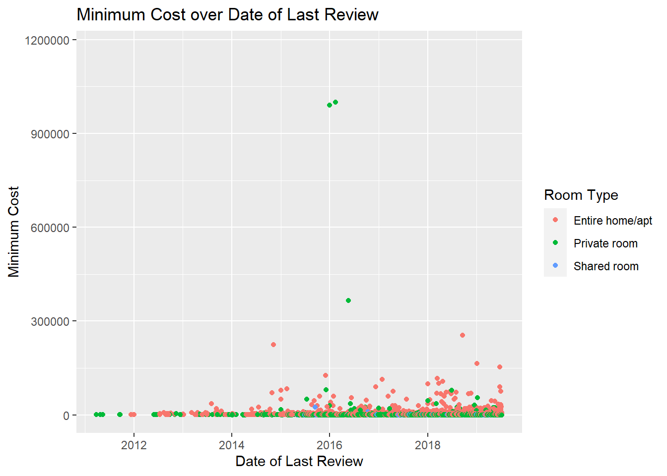
library(tidyverse)library(ggplot2)AirbnbNYC <- AB_NYC_2019 %>%mutate(`minimum_cost`=`price`*`minimum_nights`)## Time Dependent Visualizationvis1a <-ggplot(AirbnbNYC, aes(x=last_review, y=minimum_cost, color=room_type)) +geom_point() +labs(y="Minimum Cost", x="Date of Last Review", color="Room Type", title ="Minimum Cost over Date of Last Review")print(vis1a)
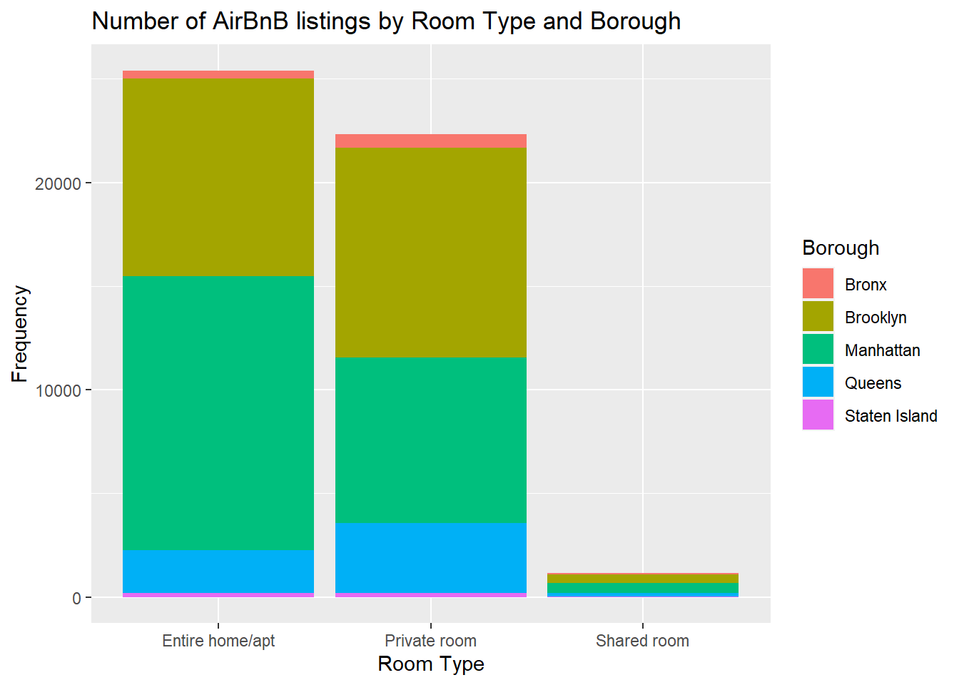
## Visualizing Part-Whole Relationshipsvis2a <-ggplot(AirbnbNYC, aes(x = room_type, fill = neighbourhood_group)) +geom_bar() +labs(y="Frequency", x="Room Type", fill ="Borough", title="Number of AirBnB listings by Room Type and Borough") print(vis2a)
Source Code
---title: "Challenge 6 Solutions"author: "Moira Chiong"description: "Visualizing Time and Relationships"date: "6/20/2023"format: html: toc: true code-copy: true code-tools: truecategories: - challenge_6 - hotel_bookings - air_bnb - fed_rate - debt - usa_households - abc_poll---```{r}setwd("C:/Users/chion/OneDrive/Desktop/DACSS 601/DACSS_601_Summer2023_Sec1/posts")library(readr)AB_NYC_2019 <-read_csv("_data/AB_NYC_2019.csv")View(AB_NYC_2019)``````{r}#| label: setup#| warning: false#| message: falselibrary(tidyverse)library(ggplot2)```## Challenge OverviewToday's challenge is to:1) read in a data set, and describe the data set using both words and any supporting information (e.g., tables, etc)2) tidy data (as needed, including sanity checks)3) mutate variables as needed (including sanity checks)4) create at least one graph including time (evolution) - try to make them "publication" ready (optional) - Explain why you choose the specific graph type5) Create at least one graph depicting part-whole or flow relationships - try to make them "publication" ready (optional) - Explain why you choose the specific graph type[R Graph Gallery](https://r-graph-gallery.com/) is a good starting point for thinking about what information is conveyed in standard graph types, and includes example R code.(be sure to only include the category tags for the data you use!)## Read in dataRead in one (or more) of the following datasets, using the correct R package and command. - debt ⭐ - fed_rate ⭐⭐ - abc_poll ⭐⭐⭐ - usa_hh ⭐⭐⭐ - hotel_bookings ⭐⭐⭐⭐ - AB_NYC ⭐⭐⭐⭐⭐### Briefly describe the dataThere are 48895 observations with 17 variables. The data set pertains to review and other administrative records for AirBnB in New York City. There are categorical variables in the data set, namely the boroughs of Brooklyn, Manhattan, Queens, Staten Island and Bronx, as well as room type: private room, entire home/apartment and shared room. The dates of the last review range from March 2011 to July 2019. The minimum cost ranges from 0 to $1.2M. The mean minimum cost is $1284.43. The composition of the lodging by room type is as follows: 52% Entire home/apartment, 46% private room and 2.4% shared room. In terms of boroughs where the Airbnb lodging is located, 2% where in the Bronx, 41% in Brooklyn, 44% in Manhattan, 12% in Queens and 1% in Staten Island. ## Tidy Data (as needed)Is your data already tidy, or is there work to be done? Be sure to anticipate your end result to provide a sanity check, and document your work here.```{r}unique(AB_NYC_2019$neighbourhood_group)proproomtype <-c(AirbnbNYC$room_type, NA)prop.table(table(AirbnbNYC$room_type))propneighgroup <-c(AirbnbNYC$neighbourhood_group, NA)prop.table((table(AirbnbNYC$neighbourhood_group)))```Are there any variables that require mutation to be usable in your analysis stream? For example, do you need to calculate new values in order to graph them? Can string values be represented numerically? Do you need to turn any variables into factors and reorder for ease of graphics and visualization?Document your work here.```{r}install.packages("tidyverse")library(tidyverse)library(ggplot2)AirbnbNYC <- AB_NYC_2019 %>%mutate(`minimum_cost`=`price`*`minimum_nights`)## Time Dependent Visualizationvis1a <-ggplot(AirbnbNYC, aes(x=last_review, y=minimum_cost, color=room_type)) +geom_point() +labs(y="Minimum Cost", x="Date of Last Review", color="Room Type", title ="Minimum Cost over Date of Last Review")print(vis1a)## Visualizing Part-Whole Relationshipsvis2a <-ggplot(AirbnbNYC, aes(x = room_type, fill = neighbourhood_group)) +geom_bar() +labs(y="Frequency", x="Room Type", fill ="Borough", title="Number of AirBnB listings by Room Type and Borough") print(vis2a)```