Code
library(tidyverse)

knitr::opts_chunk$set(echo = TRUE)library(tidyverse)
knitr::opts_chunk$set(echo = TRUE)The dataset used for analysis is the Hotel Bookings dataset which is available on Kaggle: https://www.kaggle.com/datasets/jessemostipak/hotel-booking-demand. It contains information about two hotel types - City Hotel and Resort hotels. For these two hotel types, it has information of customer arrival, checkout details, number of adults, children and babies along with their booking details, payment types, and reservation information. The data captures hotel bookings made from July 2015 to July 2017 that is 2 years of data. It provides insights into various aspects of hotel stays, such as lead time (the duration between booking and arrival), meal preferences, market segments through which bookings are made, cancellations, and tourist patterns.
hotel_bookings <- read_csv("_data/hotel_bookings.csv")Rows: 119390 Columns: 32
── Column specification ────────────────────────────────────────────────────────
Delimiter: ","
chr (13): hotel, arrival_date_month, meal, country, market_segment, distrib...
dbl (18): is_canceled, lead_time, arrival_date_year, arrival_date_week_numb...
date (1): reservation_status_date
ℹ Use `spec()` to retrieve the full column specification for this data.
ℹ Specify the column types or set `show_col_types = FALSE` to quiet this message.hotel_bookingsglimpse(hotel_bookings)Rows: 119,390
Columns: 32
$ hotel <chr> "Resort Hotel", "Resort Hotel", "Resort…
$ is_canceled <dbl> 0, 0, 0, 0, 0, 0, 0, 0, 1, 1, 1, 0, 0, …
$ lead_time <dbl> 342, 737, 7, 13, 14, 14, 0, 9, 85, 75, …
$ arrival_date_year <dbl> 2015, 2015, 2015, 2015, 2015, 2015, 201…
$ arrival_date_month <chr> "July", "July", "July", "July", "July",…
$ arrival_date_week_number <dbl> 27, 27, 27, 27, 27, 27, 27, 27, 27, 27,…
$ arrival_date_day_of_month <dbl> 1, 1, 1, 1, 1, 1, 1, 1, 1, 1, 1, 1, 1, …
$ stays_in_weekend_nights <dbl> 0, 0, 0, 0, 0, 0, 0, 0, 0, 0, 0, 0, 0, …
$ stays_in_week_nights <dbl> 0, 0, 1, 1, 2, 2, 2, 2, 3, 3, 4, 4, 4, …
$ adults <dbl> 2, 2, 1, 1, 2, 2, 2, 2, 2, 2, 2, 2, 2, …
$ children <dbl> 0, 0, 0, 0, 0, 0, 0, 0, 0, 0, 0, 0, 0, …
$ babies <dbl> 0, 0, 0, 0, 0, 0, 0, 0, 0, 0, 0, 0, 0, …
$ meal <chr> "BB", "BB", "BB", "BB", "BB", "BB", "BB…
$ country <chr> "PRT", "PRT", "GBR", "GBR", "GBR", "GBR…
$ market_segment <chr> "Direct", "Direct", "Direct", "Corporat…
$ distribution_channel <chr> "Direct", "Direct", "Direct", "Corporat…
$ is_repeated_guest <dbl> 0, 0, 0, 0, 0, 0, 0, 0, 0, 0, 0, 0, 0, …
$ previous_cancellations <dbl> 0, 0, 0, 0, 0, 0, 0, 0, 0, 0, 0, 0, 0, …
$ previous_bookings_not_canceled <dbl> 0, 0, 0, 0, 0, 0, 0, 0, 0, 0, 0, 0, 0, …
$ reserved_room_type <chr> "C", "C", "A", "A", "A", "A", "C", "C",…
$ assigned_room_type <chr> "C", "C", "C", "A", "A", "A", "C", "C",…
$ booking_changes <dbl> 3, 4, 0, 0, 0, 0, 0, 0, 0, 0, 0, 0, 0, …
$ deposit_type <chr> "No Deposit", "No Deposit", "No Deposit…
$ agent <chr> "NULL", "NULL", "NULL", "304", "240", "…
$ company <chr> "NULL", "NULL", "NULL", "NULL", "NULL",…
$ days_in_waiting_list <dbl> 0, 0, 0, 0, 0, 0, 0, 0, 0, 0, 0, 0, 0, …
$ customer_type <chr> "Transient", "Transient", "Transient", …
$ adr <dbl> 0.00, 0.00, 75.00, 75.00, 98.00, 98.00,…
$ required_car_parking_spaces <dbl> 0, 0, 0, 0, 0, 0, 0, 0, 0, 0, 0, 0, 0, …
$ total_of_special_requests <dbl> 0, 0, 0, 0, 1, 1, 0, 1, 1, 0, 0, 0, 3, …
$ reservation_status <chr> "Check-Out", "Check-Out", "Check-Out", …
$ reservation_status_date <date> 2015-07-01, 2015-07-01, 2015-07-02, 20…I created visualizations to analyze different aspects of the dataset. The lead time analysis compared lead times for Resort hotels and City hotels, revealing that City hotels had slightly higher lead times.
Market segments were also analyzed, and it was found that most bookings came from the “Online TA” (Online Travel Agents) and “Offline TA/TO” (Offline Travel Agents/Tour Operators) segments.
Furthermore, the number of cancellations and bookings per year was plotted, revealing that 2016 had the highest number of cancellations and bookings. The frequency of tourist arrivals by month was also visualized, highlighting June and August as peak months.
These analyses provide valuable insights into the hotel booking dataset, offering information about lead times, meal preferences, market segments, cancellations, and tourist patterns. The dataset was cleaned, and the results were presented using visualizations to aid in understanding the data.
I also checked the top 5 which countries most people travel from to these hotels to market accordingly. We can see that most number of travellers are from PRT - Portugal followed by GBR - United Kingdom.
country_data <- hotel_bookings %>% group_by(country) %>% count()

country_data <- head(arrange(country_data, desc(n)),5)

ggplot(data = country_data, aes(x = country, y = n,  fill = country)) +
  geom_bar(stat = "identity") +
  labs(title = "Top 5 countries", x = "Country", y = "Number of travellers")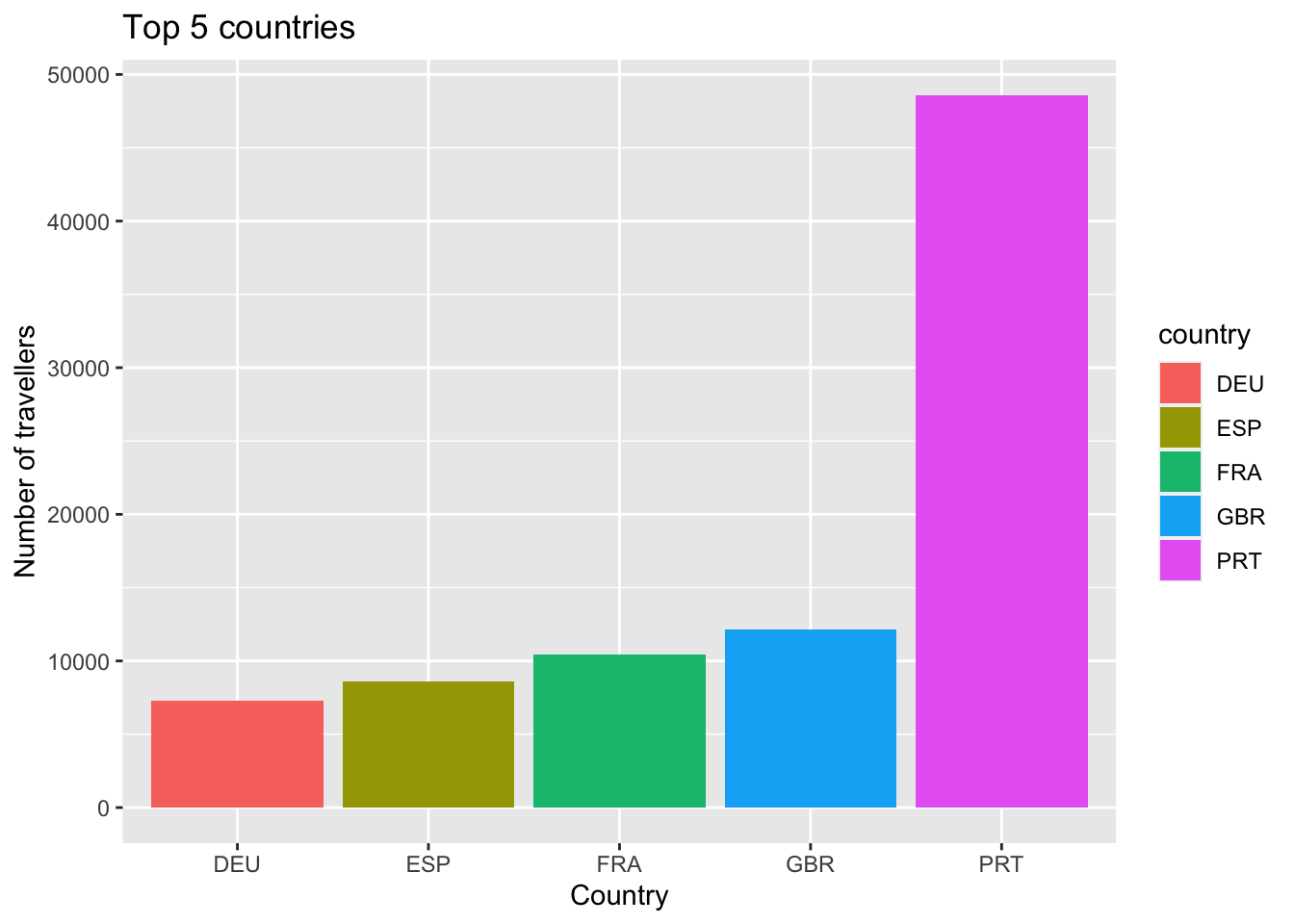
We can now start cleaning the dataset. I will be checking if any columns have missing values, null values and remove irrelavent columns. I will also rename certain list of values or column names if needed to make the dataset more readable. I will also use data visualization to understand the data better.
count_missing <- sum(is.na(hotel_bookings))
hotel_bookings <- hotel_bookings[complete.cases(hotel_bookings),]When working with datasets, it is common practice to evaluate the usefulness and relevance of each column. Columns with a high percentage of missing or irrelevant data may not contribute significantly to the analysis and and thus I am safely dropping it to simplify the dataset and focus on more informative variables.
head(hotel_bookings)table(hotel_bookings$company)
    10    100    101    102    103    104    105    106    107    108    109
     1      1      1      1     16      1      8      2      9     11      1
    11    110    112    113    115    116    118     12    120    122    126
     1     52     13     36      4      6      7     14     14     18      1
   127    130    132    135    137    139     14    140    142    143    144
    15     12      1     66      4      3      9      1      1     17     27
   146    148    149    150    153    154    158    159     16    160    163
     3     37      5     19    215    133      2      6      5      1     17
   165    167    168    169    174    178    179     18    180    183    184
     3      7      2     65    149     27     24      1      5     16      1
   185    186    192    193    195    197     20    200    202    203    204
     4     12      4     16     38     47     50      3     38     13     34
   207    209    210    212    213    215    216    217    218    219     22
     9     19      2      1      1      8     21      2     43    141      6
   220    221    222    223    224    225    227    229    230    232    233
     4     27      2    784      3      7     24      1      3      2    114
   234    237    238    240    242    243    245    246    250    251    253
     1      1     33      3     62      2      3      3      2     18      1
   254    255    257    258    259    260    263    264    268    269    270
    10      6      1      1      2      3     14      2     14     33     43
   271    272    273    274    275    277    278    279     28    280    281
     2      3      1     14      3      5      2      8      5     48    138
   282    284    286    287    288    289     29    290    291    292    293
     4      1     21      5      1      2      2     17     12     18      5
   297    301    302    304    305    307    308    309     31    311    312
     7      1      5      2      1     36     33      1     17      2      3
   313    314    316    317    318    319     32    320    321    323    324
     1      1      2      9      1      3      1      1      2     10      9
   325    329    330    331    332    333    334    337    338     34    341
     2     12      4     61      2     11      3     25     12      8      5
   342    343    346    347    348    349     35    350    351    352    353
    48     29     14      1     59      2      1      3      2      1      4
   355    356    357    358    360    361    362    364    365    366    367
    13     10      5      7     12      2      2      6     29     24     14
   368    369     37    370    371    372    373    376    377    378    379
     1      5     10      2     11      3      1      1      5      3      9
    38    380    382    383    384    385    386    388     39    390    391
    51     12      5      6      9     30      1      7      8     13      2
   392    393    394    395    396    397    398    399     40    400    401
     4      1      6      4     18     15      1     11    927      2      1
   402    403    405    407    408    409    410    411    412    413    415
     1      2    119     22     15     12      5      2      1      1      1
   416    417    418    419     42    420    421    422    423    424    425
     1      1     25      1      5      1      9      1      2     24      1
   426    428    429     43    433    435    436    437    439    442    443
     4     13      2     29      2     12      2      7      6      1      5
   444    445    446    447    448     45    450    451    452    454    455
     5      4      1      2      4    250     10      6      4      1      1
   456    457    458    459     46    460    461    465    466     47    470
     2      3      2      5     26      3      1     12      3     72      5
   477    478    479     48    481    482    483    484    485    486    487
    23      2      1      5      1      2      2      2     14      2      1
   489     49    490    491    492    494    496    497    498    499    501
     1      5      5      2      2      4      1      1     58      1      1
   504    506    507     51    511    512    513    514    515    516    518
    11      1     23     99      6      3      2      2      6      1      2
    52    520    521    523    525    528     53    530    531    534    539
     2      1      7     19     15      2      8      5      1      2      2
    54    541    543     59      6     61     62     64     65     67     68
     1      1      2      7      1      2     47      1      1    267     46
    71     72     73     76     77     78      8     80     81     82     83
     2     30      3      1      1     22      1      1     23     14      9
    84     85     86     88      9     91     92     93     94     96     99
     3      2     32     22     37     48     13      3     87      1     12
  NULL
112589 hotel_bookings <- hotel_bookings[, -which(names(hotel_bookings) == "company")]
glimpse(hotel_bookings)Rows: 119,386
Columns: 31
$ hotel <chr> "Resort Hotel", "Resort Hotel", "Resort…
$ is_canceled <dbl> 0, 0, 0, 0, 0, 0, 0, 0, 1, 1, 1, 0, 0, …
$ lead_time <dbl> 342, 737, 7, 13, 14, 14, 0, 9, 85, 75, …
$ arrival_date_year <dbl> 2015, 2015, 2015, 2015, 2015, 2015, 201…
$ arrival_date_month <chr> "July", "July", "July", "July", "July",…
$ arrival_date_week_number <dbl> 27, 27, 27, 27, 27, 27, 27, 27, 27, 27,…
$ arrival_date_day_of_month <dbl> 1, 1, 1, 1, 1, 1, 1, 1, 1, 1, 1, 1, 1, …
$ stays_in_weekend_nights <dbl> 0, 0, 0, 0, 0, 0, 0, 0, 0, 0, 0, 0, 0, …
$ stays_in_week_nights <dbl> 0, 0, 1, 1, 2, 2, 2, 2, 3, 3, 4, 4, 4, …
$ adults <dbl> 2, 2, 1, 1, 2, 2, 2, 2, 2, 2, 2, 2, 2, …
$ children <dbl> 0, 0, 0, 0, 0, 0, 0, 0, 0, 0, 0, 0, 0, …
$ babies <dbl> 0, 0, 0, 0, 0, 0, 0, 0, 0, 0, 0, 0, 0, …
$ meal <chr> "BB", "BB", "BB", "BB", "BB", "BB", "BB…
$ country <chr> "PRT", "PRT", "GBR", "GBR", "GBR", "GBR…
$ market_segment <chr> "Direct", "Direct", "Direct", "Corporat…
$ distribution_channel <chr> "Direct", "Direct", "Direct", "Corporat…
$ is_repeated_guest <dbl> 0, 0, 0, 0, 0, 0, 0, 0, 0, 0, 0, 0, 0, …
$ previous_cancellations <dbl> 0, 0, 0, 0, 0, 0, 0, 0, 0, 0, 0, 0, 0, …
$ previous_bookings_not_canceled <dbl> 0, 0, 0, 0, 0, 0, 0, 0, 0, 0, 0, 0, 0, …
$ reserved_room_type <chr> "C", "C", "A", "A", "A", "A", "C", "C",…
$ assigned_room_type <chr> "C", "C", "C", "A", "A", "A", "C", "C",…
$ booking_changes <dbl> 3, 4, 0, 0, 0, 0, 0, 0, 0, 0, 0, 0, 0, …
$ deposit_type <chr> "No Deposit", "No Deposit", "No Deposit…
$ agent <chr> "NULL", "NULL", "NULL", "304", "240", "…
$ days_in_waiting_list <dbl> 0, 0, 0, 0, 0, 0, 0, 0, 0, 0, 0, 0, 0, …
$ customer_type <chr> "Transient", "Transient", "Transient", …
$ adr <dbl> 0.00, 0.00, 75.00, 75.00, 98.00, 98.00,…
$ required_car_parking_spaces <dbl> 0, 0, 0, 0, 0, 0, 0, 0, 0, 0, 0, 0, 0, …
$ total_of_special_requests <dbl> 0, 0, 0, 0, 1, 1, 0, 1, 1, 0, 0, 0, 3, …
$ reservation_status <chr> "Check-Out", "Check-Out", "Check-Out", …
$ reservation_status_date <date> 2015-07-01, 2015-07-01, 2015-07-02, 20…replace_values <- function(data, column_name, old_value, new_value) {
data[[column_name]][data[[column_name]] == old_value] <- new_value
return(data)
}
hotel_bookings <- replace_values(hotel_bookings,"meal","BB", "Bed and Breakfast")
hotel_bookings <- replace_values(hotel_bookings,"meal","HB", "Half Board")
hotel_bookings <- replace_values(hotel_bookings,"meal","FB", "Full Board")
hotel_bookings <- replace_values(hotel_bookings,"meal","SC", "Self Catering")
hotel_bookings <- replace_values(hotel_bookings,"market_segment","Online TA", "Online Travel Agent")
hotel_bookings <- replace_values(hotel_bookings,"market_segment","Offline TA/TO", "Offline Travel Agent/Tour Operator")
hotel_bookings <- replace_values(hotel_bookings,"distribution_channel","TA/TO", "Travel Agent/Tour Operator")
hotel_bookings <- replace_values(hotel_bookings,"distribution_channel","GDS", "Global Distribution System")
hotel_bookings <- hotel_bookings %>%
mutate(cancel_status = ifelse(is_canceled == 1, "Canceled", "Not Canceled"))The distribution of meal types chosen by guests was visualized using a pie chart, with “Bed and Breakfast” being the most common choice. I created a pie chart of meal types and based on the analysis of the pie chart of meal types, we can observe the following insights:
Most people opt for “Bed and Breakfast” in hotels: The largest slice in the pie chart represents the “Bed and Breakfast” meal type. This indicates that a significant portion of hotel guests prefer a meal plan that includes breakfast. This preference could be due to the convenience and cost-effectiveness of having breakfast provided by the hotel.
Complimentary breakfast may influence the choice of meal type: One possible explanation for the popularity of the “Bed and Breakfast” meal type is that many hotels offer complimentary breakfast as part of their services. This complimentary offering can attract guests and make the “Bed and Breakfast” option more appealing.
“Half board” and “Self catering” are also chosen by guests: The second and third largest slices in the pie chart represent the “Half board” and “Self catering” meal types, respectively. This suggests that a considerable number of guests opt for meal plans that include either breakfast and dinner or prefer to make their own meal arrangements. These options provide flexibility for guests who may have specific dietary requirements or prefer to explore local dining options.
Fewer guests choose “Full board”: The smaller slice in the pie chart represents the “Full board” meal type. This option, which includes all meals provided by the hotel, is chosen by a relatively smaller number of guests. It indicates that the majority of guests prefer meal plans that offer more flexibility or that they may dine outside the hotel for some of their meals.
ggplot(hotel_bookings, aes(x = "", fill = meal)) +
  geom_bar(size = 1, alpha = 0.8) +
  coord_polar("y", start=0) +
  scale_fill_brewer("Meal type") +
  theme_void() +
  labs(title = "Meal Preferences",
       subtitle = "Hotel Booking Dataset") +
  theme_minimal()
Warning: Using `size` aesthetic for lines was deprecated in ggplot2 3.4.0.
ℹ Please use `linewidth` instead.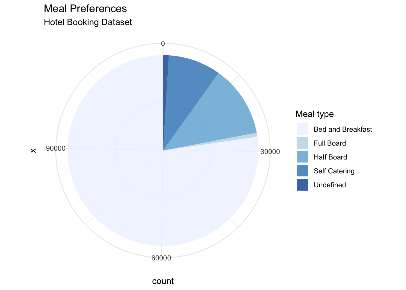
Q1. Which factors affect the lead time? What is the average lead time and does it depend on people having children or hotel type?
From the summary, we can observe that the mean lead time for hotel bookings is approximately 104 days, suggesting that people, on average, tend to book their stays approximately 3 to 3.5 months in advance. This information prompted me to investigate whether the lead time differs between Resort hotels and City hotels.
Initially, my hypothesis was that the lead time would be higher for Resort hotels, assuming that people tend to book their vacations well in advance. On the other hand, I thought that City hotels could be booked due to office work or immediate needs, potentially resulting in shorter lead times. However, upon analyzing the lead time data for both hotel types, I discovered that my hypothesis was incorrect. Surprisingly, the lead time for City hotels was slightly higher than for Resort hotels. It is worth noting that there was a significant difference in the amount of data available for City hotels compared to Resort hotels, with City hotels having almost twice as much data. This uneven distribution of data may have influenced the lead time analysis, making it difficult to draw definitive conclusions about the relationship between lead time and hotel type.
lead_time_summary <- hotel_bookings %>%
  group_by(hotel) %>%
  summarize('mean_lead_time' = mean(lead_time), 'max_lead_time' = max(lead_time), 'min_lead_time' = min(lead_time))


ggplot(data = lead_time_summary, aes(x = mean_lead_time, y = hotel)) +
  # Specify the type of plot and customize it as needed
  geom_col(fill = "blue") +
  labs(title = "Hotel type vs Lead Time", x = "Lead time", y = "Hotel type")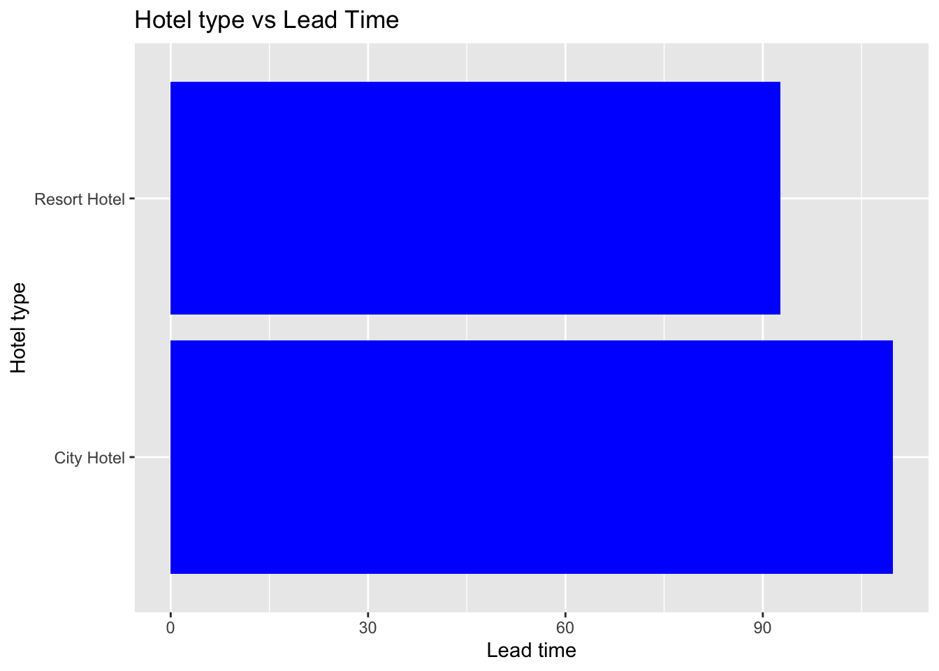
hotel_type_summary <- hotel_bookings %>%
  group_by(hotel) %>% count()

hotel_type_summary
To provide a clearer comparison between the lead time distributions of City hotels and Resort hotels, I created histograms for both individually. I separated the histograms by hotel type, allowing for a direct visual comparison of the distributions. Additionally, I included vertical dashed lines on the histograms to represent the mean lead time for each hotel type.
This updated visualization provides a better understanding of the lead time distributions for City hotels and Resort hotels, enabling comparison of the shapes of the distributions and identify any differences. By incorporating the mean lead time lines on the histograms, we can easily compare the central tendencies of the distributions.
In summary, my analysis revealed that the lead time for City hotels was slightly higher than for Resort hotels, contradicting my initial hypothesis. However, it is important to consider the limitations and data distribution when interpreting these results concerning lead time and hotel type.
lead_time_comparison <- hotel_bookings %>%
  mutate(hotel = factor(hotel, levels = c("City Hotel", "Resort Hotel")))


ggplot(data = lead_time_comparison, aes(x = lead_time)) +
  geom_histogram(fill = "blue", color = "black", bins = 30) +
  facet_grid(hotel ~ ., scales = "free_y") +
  geom_vline(data = lead_time_summary, aes(xintercept = mean_lead_time),
             color = "red", linetype = "dashed", size = 1) +
  labs(title = "Lead Time Distribution by Hotel Type",
       x = "Lead Time", y = "Frequency") +
  theme_bw()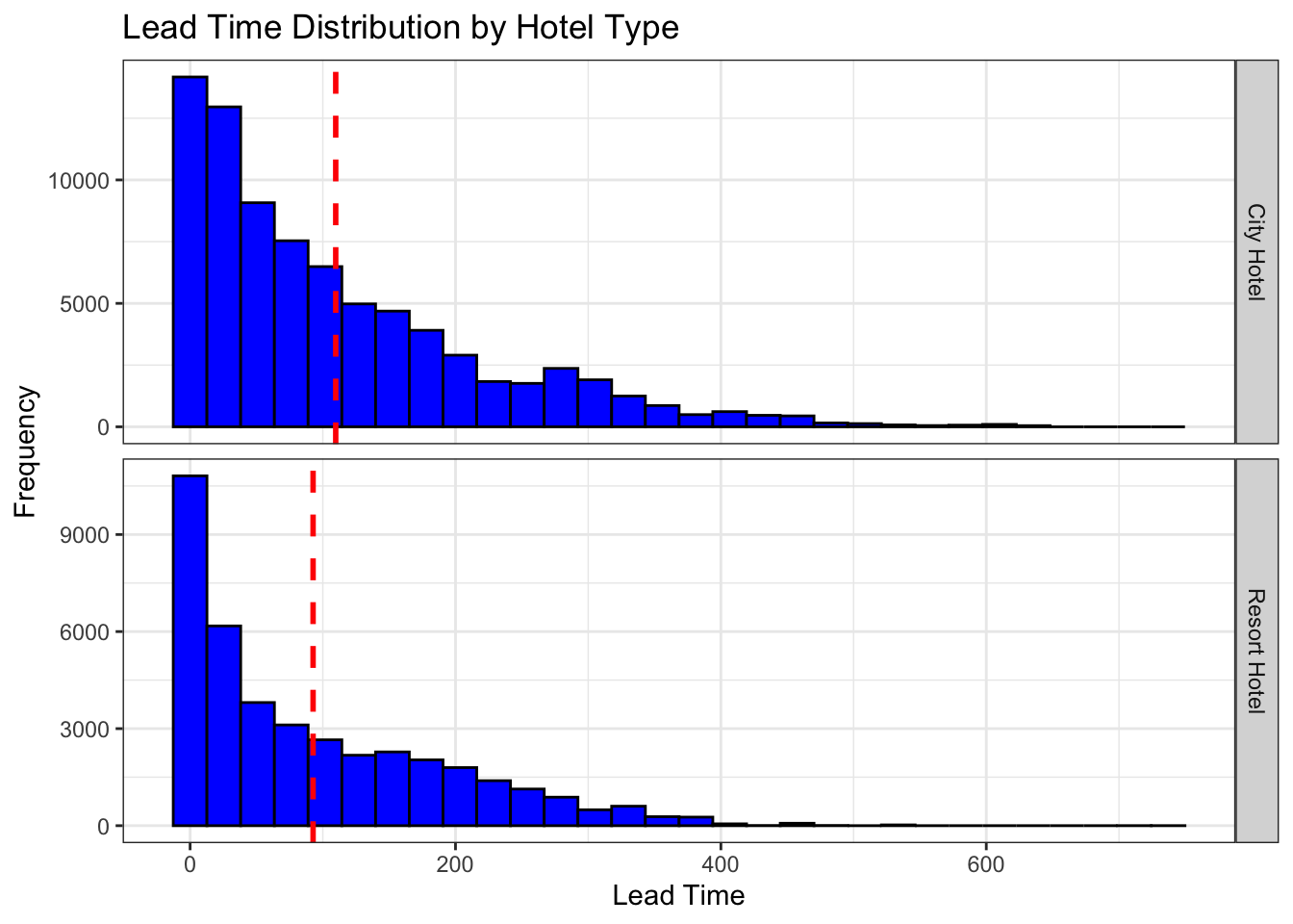
We can instead check if Lead time is affected by people having children. The graph titled “Median Lead Time by Number of Children” provides insights into the relationship between the number of children and the median lead time for hotel bookings. The median lead time is a measure of central tendency that represents the middle value of the lead times for a given group of bookings with the same number of children. We can see that the median lead time varies from 55 to 70 days overall for people with or without any children. Thus we cannot say for sure if there is any pattern here.
children_lead_time_summary <- hotel_bookings %>%
  group_by(children) %>%
  summarize(median_lead_time = median(lead_time, na.rm = TRUE))

ggplot(data = children_lead_time_summary, aes(x = children, y = median_lead_time)) +
  geom_bar(stat = "identity", fill = "blue", color = "black") +
  labs(title = "Median Lead Time by Number of Children", x = "Number of Children", y = "Median Lead Time")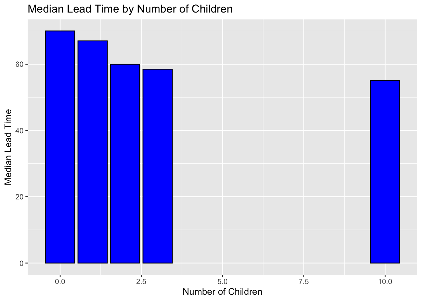
Q2 What are the factors affecting the cancellation of hotel bookings? Does it depend on hotel type, seasonal trends or the deposit type through which the bookings are taken? Can the hotels try to take extra bookings accordingly if there is a pattern in booking cancellations based on these factors?
To start with, I created a plot of cancellations per year and we can see that 2016 had the most number of cancellations as well as bookings.To check if there is any trend in cancellations based on market segment I also created that distribution. We can see that most of the bookings came from Online TA market segment and so did the cancellations.Thus it seems to be in sync and no particular trend based on market segment.
is_categorical <- class(hotel_bookings$cancel_status) == "factor" || is.character(hotel_bookings$cancel_status)

# Convert to categorical if not already
if (!is_categorical) {
  hotel_bookings$cancel_status <- as.factor(hotel_bookings$cancel_status)
}

hotel_bookings%>%

  ggplot(aes(x=arrival_date_year,fill=cancel_status)) + geom_bar()+
  labs(title = "Booking Cancellation by year", x = "Year", y = "Number of bookings", fill ='Booking Status')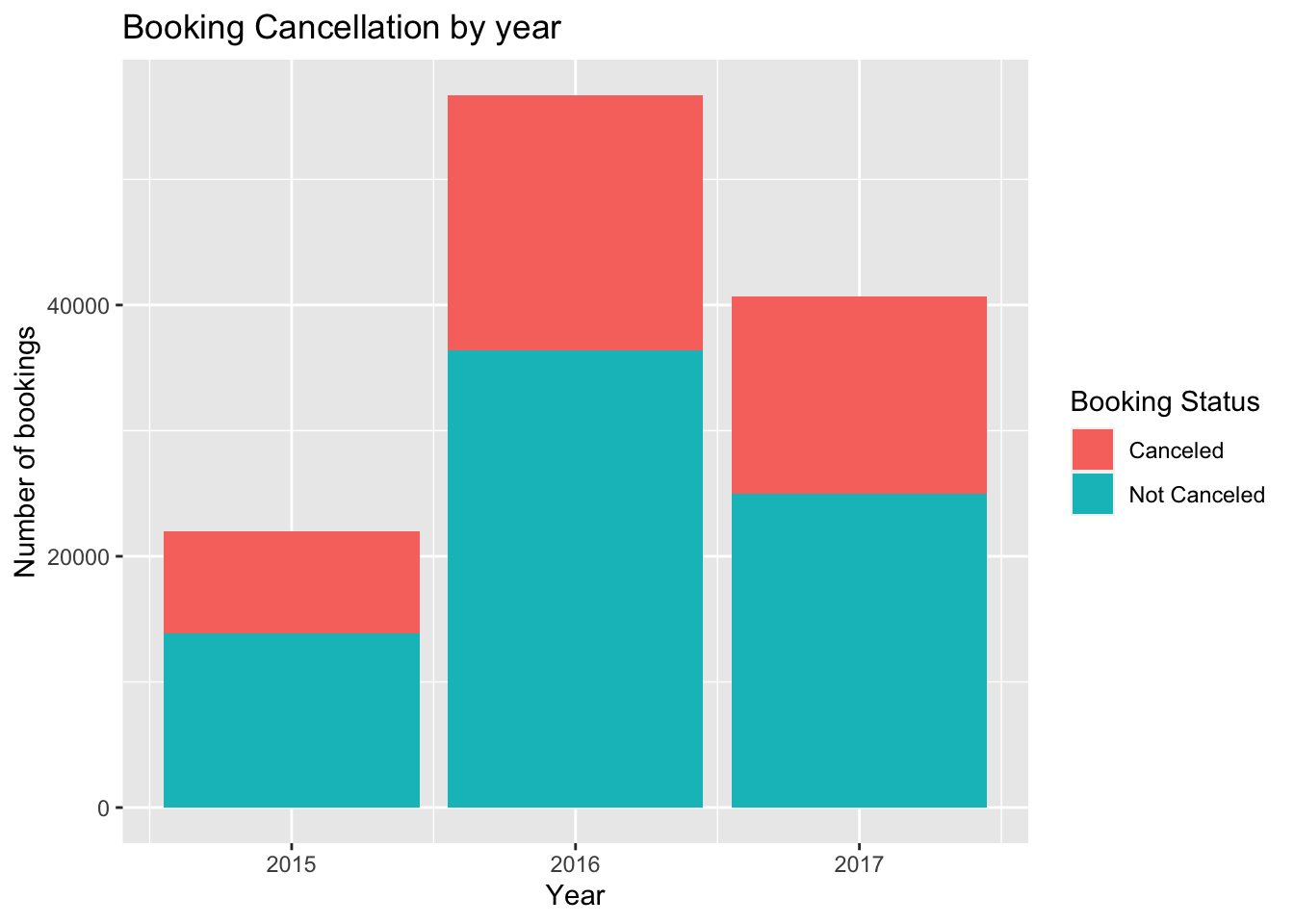
hotel_bookings %>%
  ggplot(mapping = aes(x=cancel_status, fill = market_segment)) +
  facet_wrap(. ~ hotel)+
  geom_bar() +
  labs(title = "Booking Satus by Hotel type and Market Segment", x = "Booking Satus", y = "Number of bookings", fill ='Market Segment')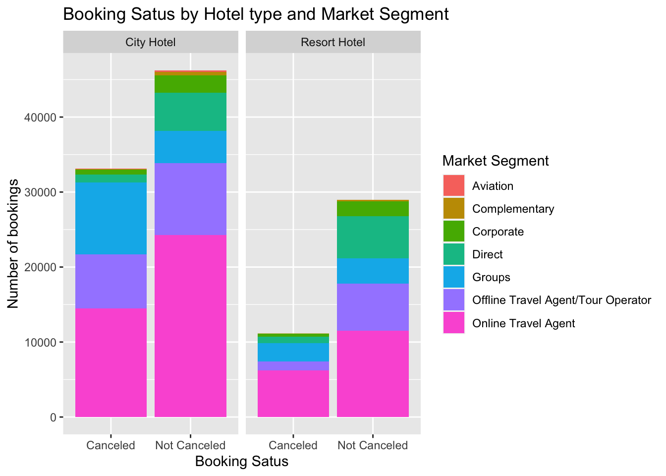
Next I want to check if the cancellations very depending on whether it is a City hotel or a Resort hotel.
Upon examining the cancellations hotel wise, it becomes apparent that the proportion of cancelled bookings differs between the two types of hotels. Specifically, for the City Hotel, the majority of bookings (58.28%) were non-cancelled, while 41.72% of the bookings were cancelled. On the other hand, for the Resort Hotel, a higher percentage (72.24%) of bookings were non-cancelled, while only 27.76% of the bookings were cancelled. It is worth noting that, although most bookings in both hotels were not cancelled, there is a notable disparity in the cancellation rates between the two hotel types.
# Calculate the cancellation percentages
hotel_summary <- hotel_bookings %>%
  group_by(hotel, cancel_status) %>%
  summarise(count = n()) %>%
  mutate(percentage = count / sum(count) * 100)
`summarise()` has grouped output by 'hotel'. You can override using the
`.groups` argument.# Create the bar plot
ggplot(data = hotel_summary, aes(x = hotel, y = percentage, fill = cancel_status)) +
geom_bar(stat = "identity", position = "fill") +
geom_text(aes(label = paste(round(percentage, 1), "%")),
position = position_fill(vjust = 0.5),
color = "white", size = 4) +
labs(title = "Cancelled vs Non-cancelled Bookings",
x = "Hotel Type",
y = "Percentage",
fill = "Booking Status") +
scale_fill_manual(values = c("#F8766D", "#00BFC4")) +
theme_minimal()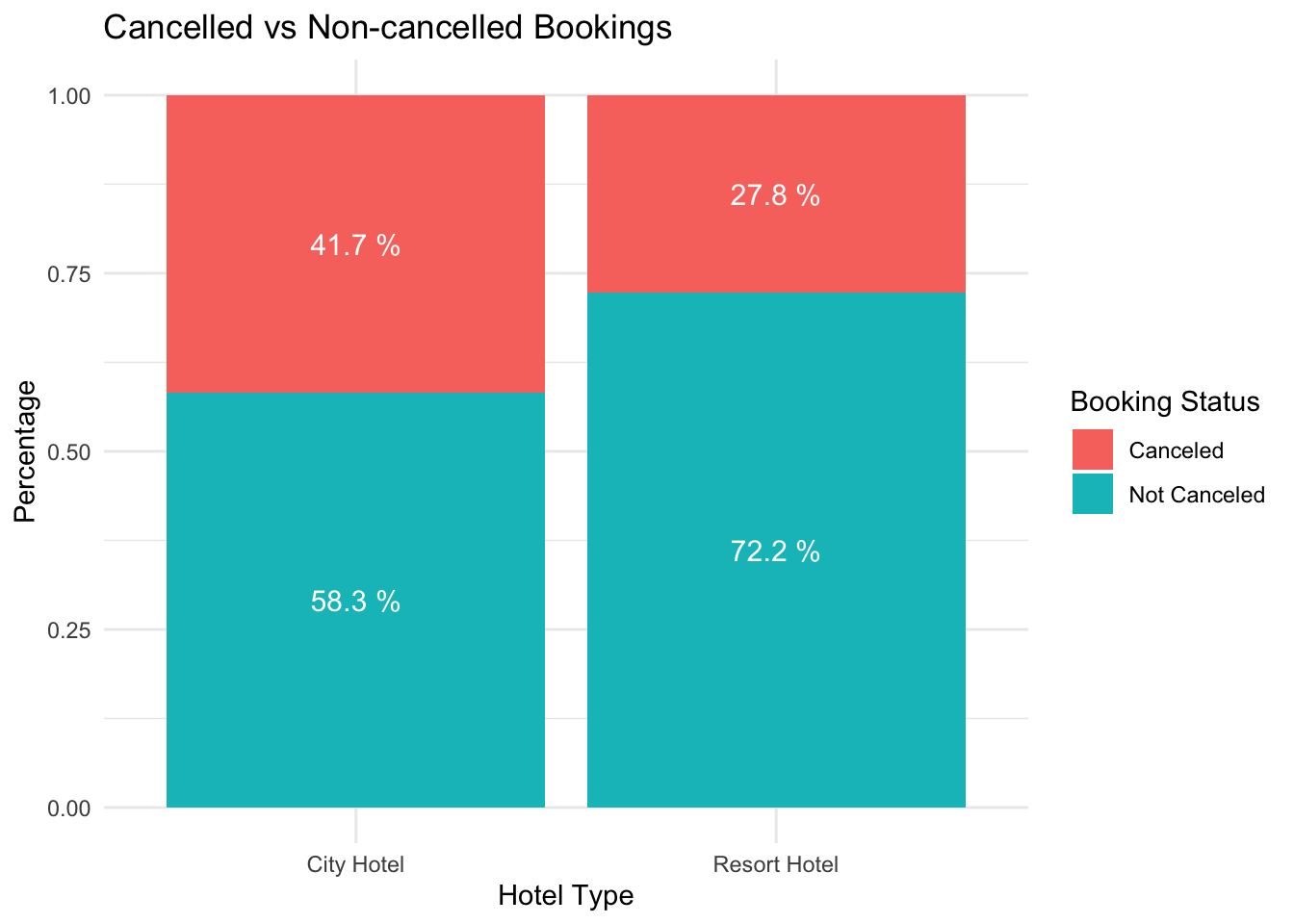
The investigation further explored cancellations based on deposit types. I hypothesized that most cancellations would be for bookings with no deposit, as people are less likely to cancel if they have already made a payment. I will check this for City Hotels first followed by Resort Hotels.
booking_summary <- hotel_bookings %>%
  select(hotel, cancel_status, deposit_type) %>%
  filter(hotel == 'City Hotel') %>%
  group_by(hotel, cancel_status, deposit_type) %>%
  summarise(number_of_bookings = n())
`summarise()` has grouped output by 'hotel', 'cancel_status'. You can override
using the `.groups` argument.ggplot(booking_summary, aes(x = deposit_type, y = number_of_bookings, fill = cancel_status)) +
geom_col(position = position_dodge2(width = 0.9), width = 0.6, color = "black") +
geom_text(aes(label = number_of_bookings),
position = position_dodge2(width = 0.9),
vjust = -0.5,
size = 3.5,
color = "black",
fontface = "bold",
check_overlap = TRUE) +
scale_fill_manual(values = c("#FF69B4", "#4169E1")) +
labs(title = "Number of Bookings by Deposit Type for City Hotels",
x = "Deposit Type",
y = "Number of Bookings") +
theme(plot.title = element_text(hjust = 0.5, size = 14, face = "bold"),
axis.title = element_text(size = 12),
axis.text = element_text(size = 10),
panel.grid.major.x = element_blank(),
legend.title = element_blank(),
legend.position = "bottom",
legend.text = element_text(size = 10)) +
guides(fill = guide_legend(reverse = TRUE))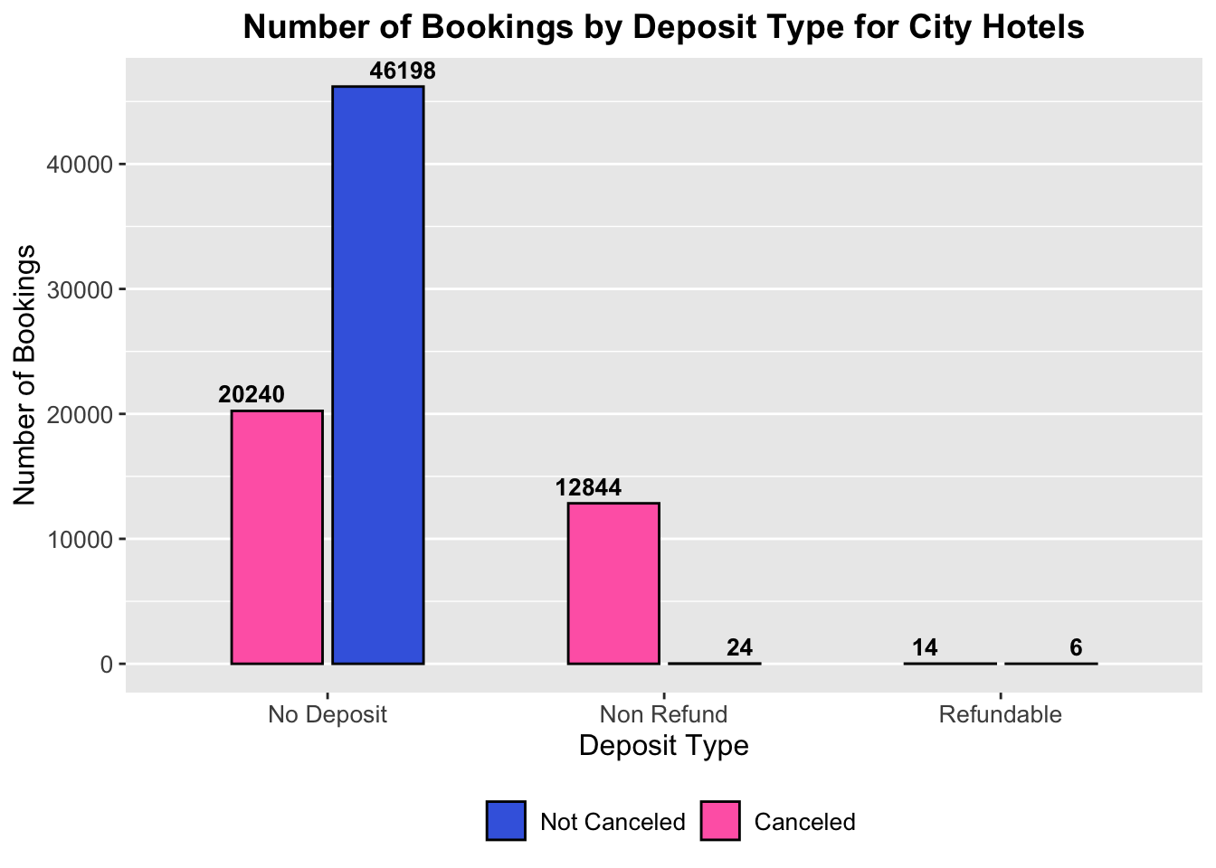
Now checking the same for Resort hotel:
booking_summary <- hotel_bookings %>%
  select(hotel, cancel_status, deposit_type) %>%
  filter(hotel == 'Resort Hotel') %>%
  group_by(hotel, cancel_status, deposit_type) %>%
  summarise(number_of_bookings = n())
`summarise()` has grouped output by 'hotel', 'cancel_status'. You can override
using the `.groups` argument.ggplot(booking_summary, aes(x = deposit_type, y = number_of_bookings, fill = cancel_status)) +
geom_col(position = position_dodge2(width = 0.9), width = 0.6, color = "black") +
geom_text(aes(label = number_of_bookings),
position = position_dodge2(width = 0.9),
vjust = -0.5,
size = 3.5,
color = "black",
fontface = "bold",
check_overlap = TRUE) +
scale_fill_manual(values = c("#FF69B4", "#4169E1")) +
labs(title = "Number of Bookings by Deposit Type for Resort Hotels",
x = "Deposit Type",
y = "Number of Bookings") +
theme(plot.title = element_text(hjust = 0.5, size = 14, face = "bold"),
axis.title = element_text(size = 12),
axis.text = element_text(size = 10),
panel.grid.major.x = element_blank(),
legend.title = element_blank(),
legend.position = "bottom",
legend.text = element_text(size = 10)) +
guides(fill = guide_legend(reverse = TRUE))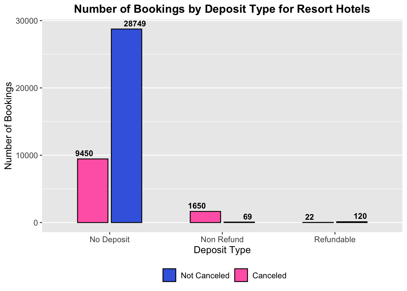
The analysis confirmed this hypothesis, as the majority of cancellations were indeed associated with bookings without any deposit. However, it was interesting to note that the Non Refundable bookings had a higher number of cancellations than expected. This indicates that even if a booking is Non Refundable, it does not guarantee that it will not be cancelled.
Let’s see the seasonal analysis of cancellation rates to see which months have highest cancellation.
hotel_bookings$month <- factor(hotel_bookings$arrival_date_month, levels = month.name)

# Calculate cancellation rates by month
cancellation_rates <- hotel_bookings %>%
  group_by(month) %>%
  summarise(cancellation_rate = sum(is_canceled) / n())


booking_rate_success <- hotel_bookings %>%
  group_by(month) %>%
  summarise(booking_rate_success = sum(!is_canceled) / n())


# Create a line plot of cancellation rates by month
ggplot(cancellation_rates, aes(x = month, y = cancellation_rate, group =1 )) +
  geom_line(color = "red") +
  labs(title = "Cancellation Rates by Month",
       x = "Month",
       y = "Cancellation Rate") +
  theme_minimal()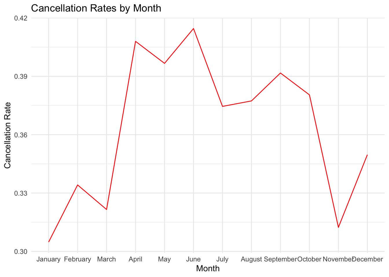
ggplot(booking_rate_success, aes(x = month, y = booking_rate_success, group =1)) +
  geom_line(color = "green") +
  labs(title = "Monthly Successful Booking Rate",
       x = "Month",
       y = "Successful Booking Rate")
Thus we can see that June has the highest cancellation rate which is 41%. June had the highest cancellation rate, possibly due to the summer vacation period when travel plans are more prone to changes. This insight highlights the importance of managing bookings during peak seasons and developing strategies to minimize cancellations during high-demand periods. January has the lowest cancellation rate of 31% followed by November.
I will combine both these charts since they are mutually exclusive sets and the sum of cancellation rate and successful booking rate any month will be equal to 1.
combined_data <- full_join(cancellation_rates, booking_rate_success, by = "month")

ggplot(combined_data, aes(x = month, group = 1)) +
  geom_line(aes(y = cancellation_rate, color = "Cancellation Rate"), size = 0.5) +
  geom_line(aes(y = booking_rate_success, color = "Booking Rate (Success)"), size = 0.5) +
  labs(title = "Monthly Rates",
       x = "Month",
       y = "Rate") +
  theme_minimal() +
  scale_color_manual(values = c("green", "red"),
                     labels = c("Booking Rate (Success)", "Cancellation Rate"),
                     name = "Rate Type") +
  scale_x_discrete(breaks = combined_data$month,
                   labels = str_sub(combined_data$month, start = 1, end = 3))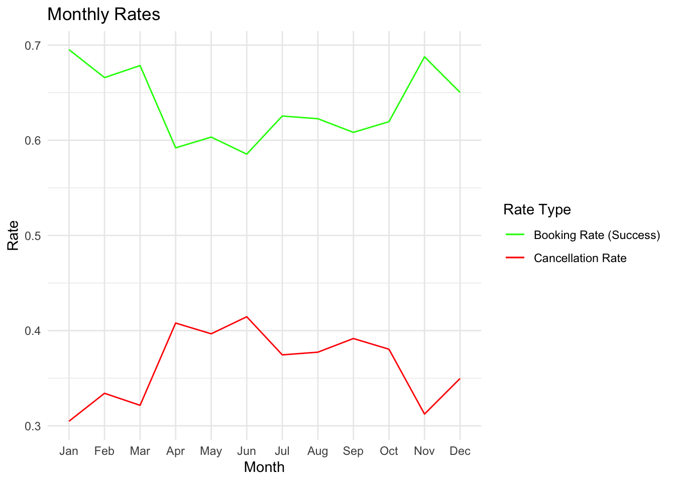
To get a comprehensive view, I combined the information from cancellation rates and successful booking rates, scaled the frequency of bookings from 0 to 1, and compared it with the cancellation rates. This enabled a clearer comparison of monthly booking frequency and cancellation rates, highlighting any correlations or patterns between the two. Interestingly, both the line graphs representing booking success rate and cancellation rates appeared as mirror images of each other.
This suggests a possible relationship between booking frequency and cancellation rates, where periods of high booking activity may also lead to higher cancellation rates.
month_counts <- as.data.frame(table(hotel_bookings$month))

colnames(month_counts) <- c("month", "Frequency")

min_val <- min(month_counts$Frequency)
max_val <- max(month_counts$Frequency)
scaled_freq <- (month_counts$Frequency - min_val) / (max_val - min_val)
scaled_df <- data.frame(month = month_counts$month, Frequency = scaled_freq)

ggplot(scaled_df, aes(x =  month, y = Frequency, group =1 )) +
  geom_line(color = "black") +
  labs(title = "Bookings by Month",
       x = "Month",
       y = "Number of Bookings") +
  theme_minimal()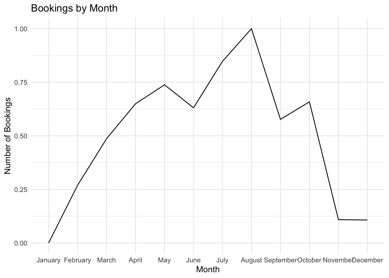
The lower number of bookings in January, December, and November indicates a seasonal trend where people tend to stay home during the winter season. This observation aligns with common travel patterns during colder months. Hoteliers can leverage this insight to develop targeted promotions and offers to attract guests during these quieter periods. Out of these bookings also January has a cancellation rate of 31%. Thus we can say that 70% people retain their bookings during winter and few cancel.
Whereas the bookings are highest from May to September peaking in August indicating that summer months are the most popular time for tourism as expected. Most people make bookings during summer out of which we saw that June had a high cancellation rate compared to other months. Thus this information can be useful to hotels suggesting that out of the summer months June will have maximum cancellations which is 41%. Thus to boom their business, the hotels can also take some extra bookings during this month as the expected cancellation rate is 41%. By allowing some extra bookings during June, hotels can compensate for the expected cancellations and avoid empty rooms or revenue loss.
We can also check for June month which has the highest cancellation rate, if the cancellations are based on deposit type. Since our previous analysis suggests that the most cancellations are made for bookings with No Deposit.
june_bookings <- hotel_bookings %>%
  filter(month == "June")

booking_summary <- june_bookings %>%
  select( cancel_status, deposit_type) %>%
  group_by(cancel_status, deposit_type) %>%
  summarise(number_of_bookings = n())
`summarise()` has grouped output by 'cancel_status'. You can override using the
`.groups` argument.ggplot(booking_summary, aes(x = deposit_type, y = number_of_bookings, fill = cancel_status)) +
geom_col(position = position_dodge2(width = 0.9), width = 0.6, color = "black") +
geom_text(aes(label = number_of_bookings),
position = position_dodge2(width = 0.9),
vjust = -0.5,
size = 3.5,
color = "black",
fontface = "bold",
check_overlap = TRUE) +
scale_fill_manual(values = c("#FF69B4", "#4169E1")) +
labs(title = "Number of Bookings in June by Deposit Type",
x = "Deposit Type",
y = "Number of Bookings in June") +
theme(plot.title = element_text(hjust = 0.5, size = 14, face = "bold"),
axis.title = element_text(size = 12),
axis.text = element_text(size = 10),
panel.grid.major.x = element_blank(),
legend.title = element_blank(),
legend.position = "bottom",
legend.text = element_text(size = 10)) +
guides(fill = guide_legend(reverse = TRUE))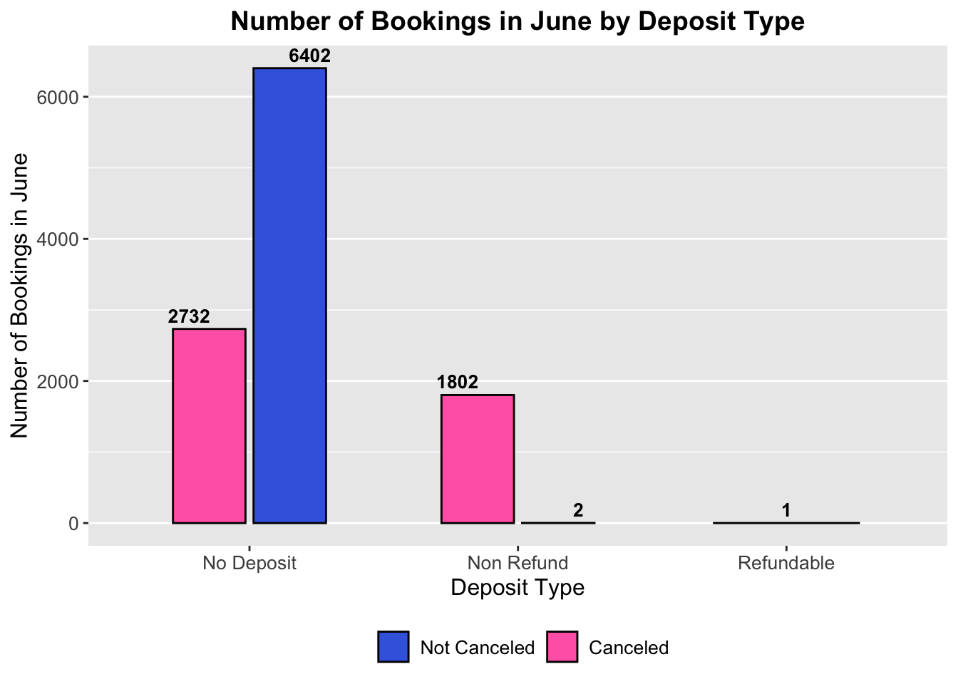
Thus we can see that bookings made by No Deposit and Non Refund both resulted in expected cancellation as per their cancellation rate. Infact cancellations seem to be higher for Non Refund deposit type.Thus we can conclude that overall June will expect a lot of cancellations and there is no fixed pattern based on Deposit type.
Next I want to check if there is any relation between lead time and hotel cancellation.
# Calculate cancellation rates by month
booking_data <- hotel_bookings %>%
  select(lead_time, is_canceled)

# Calculate the cancellation rate based on lead time
cancellation_rate <- booking_data %>%
  group_by(lead_time) %>%
  summarise(cancellation_rate = mean(is_canceled))


# Create a scatter plot of lead time vs. cancellation rate
ggplot(cancellation_rate, aes(x = lead_time, y = cancellation_rate)) +
  geom_point() +
  geom_smooth(method = "lm", se = FALSE) +
  labs(title = "Cancellation Rate vs. Lead Time",
       x = "Lead Time (days)",
       y = "Cancellation Rate") +
  theme_minimal()
`geom_smooth()` using formula = 'y ~ x'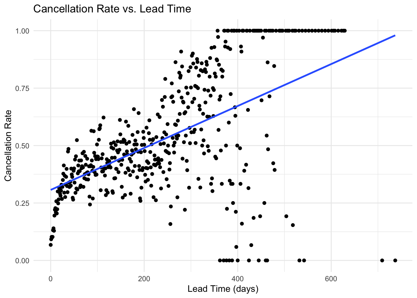
We can see that the cancellation rate increases with lead time. Thus if people booking their hotel stays very much in advance the more likely they are to cancel. Any lead time above 300 days has more than 50% chances of cancellation. This can be another important factor to consider when predicting cancellations for hotel bookings.
In conclusion, the analysis of cancellations in the hotel bookings dataset revealed valuable insights for hotel management. Understanding trends in cancellations based on factors such as market segment, hotel type, deposit types, and seasonality can help hotels optimize their booking strategies, manage revenue, and make informed decisions to mitigate cancellations.
Q3. How does market segment and distribution channel affect the hotel booking? What promotion strategies can we make based on the above two factors?
In exploring the hotel booking data, I begin by examining the popularity of different distribution channels. It is evident that the majority of bookings came through Travel Agents and Tour Operators, followed by Direct bookings and Corporate bookings. This suggests that customers often rely on the expertise and convenience provided by Travel Agents when making their reservations, while Direct bookings offer a more independent approach.
ggplot(data = hotel_bookings) +
  geom_bar(mapping = aes(x = distribution_channel, fill = distribution_channel)) +
  scale_x_discrete(labels = function(x) str_wrap(x, width = 15)) +
    labs(title='Distribution Channel wise Booking Frequency', x='Distribution Channel', y='Number of Bookings', fill = 'Distribution channel')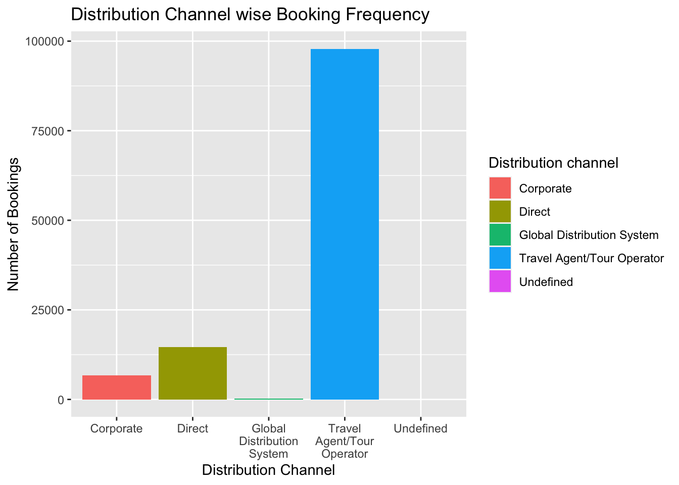
To gain further insights, I investigate the alignment between distribution channels and market segments. Notably, the Travel Agent/Tour Operator channel exhibits a strong association with customers who prefer booking through Online or Offline Travel Agents. Additionally, the Group segment shows a significant presence within this channel, as organizing bookings for a large number of people is often facilitated by Travel Agents. Similarly, Direct bookings are favored by individuals who prefer making their reservations directly, potentially seeking more control and flexibility in their arrangements.
ggplot(data=hotel_bookings) +
    geom_bar(mapping=aes(x=distribution_channel, fill=market_segment)) +
  scale_x_discrete(labels = function(x) str_wrap(x, width = 15)) +
    labs(title='Market Segment vs. Distribution Channel', x='Distribution Channel', y='Market Segment Proportion', fill = 'Market Segment')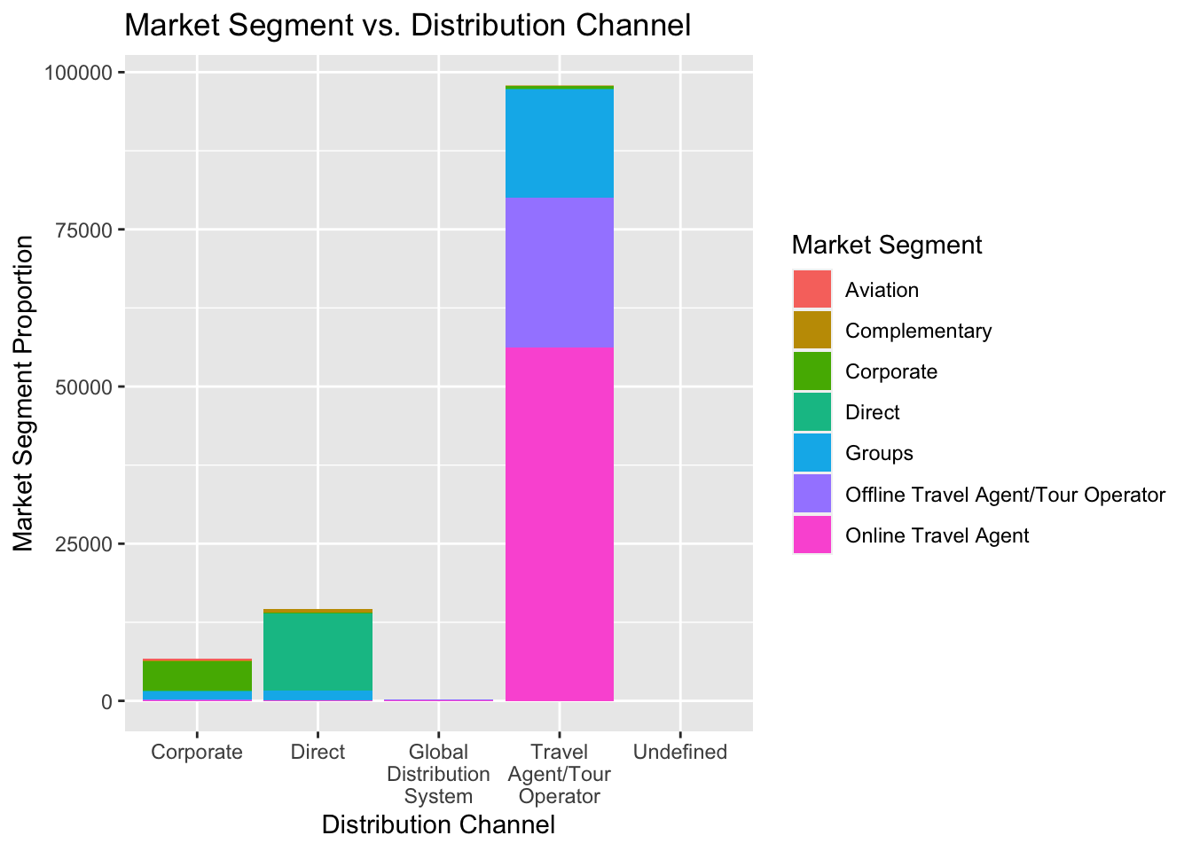
Next I want to analyze the Cancellation rates for each Distribution channel.
# Calculate cancellation rate by market segment
cancellation_rate_channel <- hotel_bookings %>%
  group_by(distribution_channel) %>%
  summarise(cancellation_rate = mean(is_canceled))


ggplot(cancellation_rate_channel, aes(x = reorder(distribution_channel, -cancellation_rate), y = cancellation_rate)) +
  geom_bar(stat = "identity", fill = "steelblue") +
  labs(title = "Cancellation Rate by Market Segment",
       x = "Market Segment",
       y = "Cancellation Rate") +
  theme_minimal() +
  coord_flip()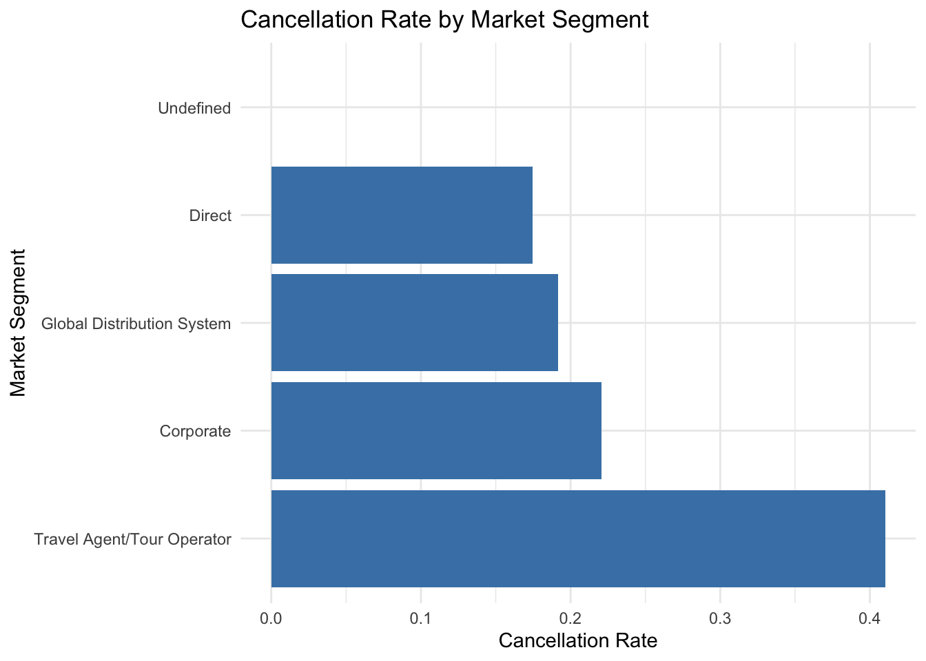
Shifting my focus to cancellation rates, I analyze the likelihood of bookings being canceled across different distribution channels. Interestingly, bookings made through Undefined channels have an alarmingly high cancellation rate of 80%, while Travel Agent bookings have a cancellation rate of 40%. However, it is important to note that Travel Agents also contribute the highest number of bookings, so a relatively higher cancellation rate is to be expected. Conversely, Direct bookings exhibit the lowest cancellation rate of approximately 18%. This indicates that customers who book directly are least likely to experience cancellations, suggesting a higher level of commitment.
We can also check if repeated guests book through the same distribution channel as non repeated guests.
hotel_bookings$is_repeated_guest <- factor(hotel_bookings$is_repeated_guest, labels = c("Non-repeated", "Repeated"))

distribution_channel_usage <- hotel_bookings %>%
  group_by(is_repeated_guest, distribution_channel) %>%
  summarise(booking_count = n()) %>%
  mutate(booking_percentage = booking_count / sum(booking_count) * 100)
`summarise()` has grouped output by 'is_repeated_guest'. You can override using
the `.groups` argument.# Create a bar plot of distribution channel usage by guest type
ggplot(distribution_channel_usage, aes(x = distribution_channel, y = booking_percentage, fill = is_repeated_guest)) +
geom_bar(stat = "identity", position = "fill") +
scale_x_discrete(labels = function(x) str_wrap(x, width = 15)) +
labs(title = "Distribution Channel Usage by Guest Type",
x = "Distribution Channel",
y = "Booking Percentage",
fill = 'Guest Type') +
scale_fill_manual(values = c("Non-repeated" = "steelblue", "Repeated" = "darkorange")) +
theme_minimal()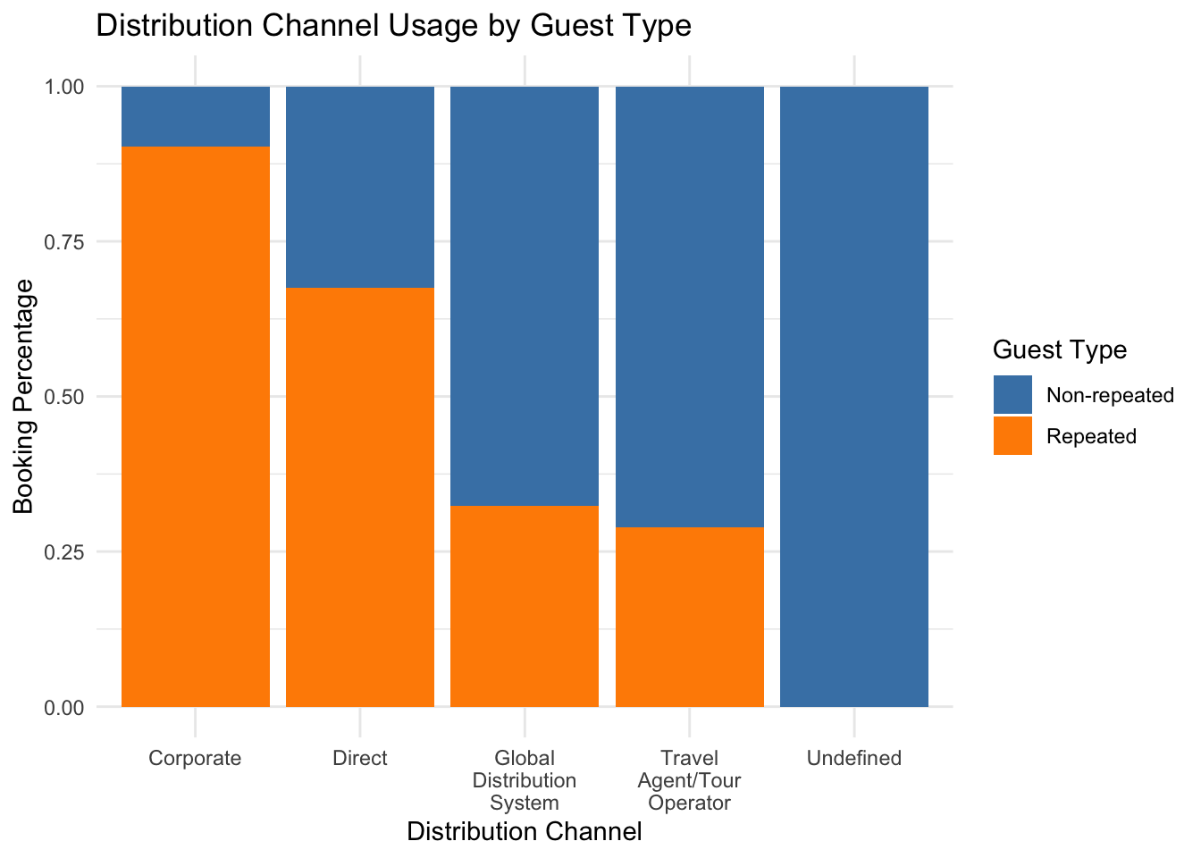
Examining the behavior of repeated guests, I uncover intriguing insights about their preferred distribution channels. Corporate bookings emerge as the primary choice for repeated guests, closely followed by Direct bookings. In contrast, Travel Agents and Undefined channels attract the least number of repeated guests. This pattern suggests that once customers have previously visited a hotel, they tend to opt for direct bookings in subsequent stays. The prevalence of repeated guests in the corporate channel may be attributed to employees frequently traveling to specific locations for work purposes.
ggplot(data = hotel_bookings) +
  geom_bar(mapping = aes(x = distribution_channel, y = booking_changes, fill = distribution_channel),
           stat = "summary", fun.y = "sum") +
  scale_x_discrete(labels = function(x) str_wrap(x, width = 15)) +
  labs(title = 'Booking Changes by Distribution Channel',
       x = 'Distribution Channel',
       y = 'Number of Booking Changes',
       fill = 'Distribution Channel')
Warning in geom_bar(mapping = aes(x = distribution_channel, y =
booking_changes, : Ignoring unknown parameters: `fun.y`No summary function supplied, defaulting to `mean_se()`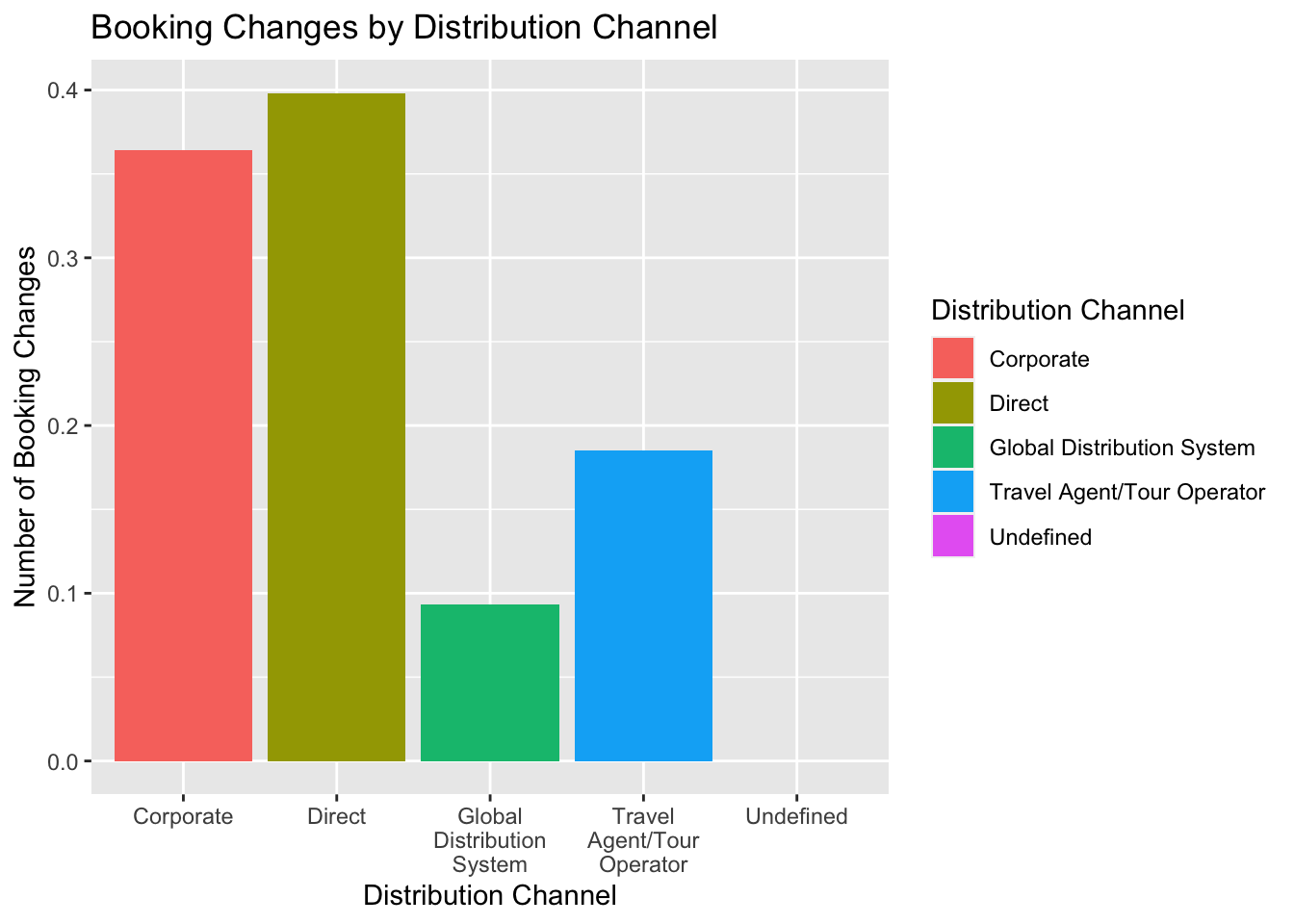
Further analysis reveals the frequency of booking changes across distribution channels. Corporate and Direct channels stand out with the highest number of booking changes. This could be attributed to factors such as corporate travel plan alterations and employee preferences, which are often covered by the company. On the other hand, Travel Agent bookings also experience a significant number of changes, possibly due to additional charges imposed by travel agents for such modifications.
ggplot(data = hotel_bookings) +
  geom_bar(mapping = aes(x = distribution_channel, y = days_in_waiting_list
, fill = distribution_channel),
           stat = "summary", fun.y = "sum") +
  scale_x_discrete(labels = function(x) str_wrap(x, width = 15)) +
  labs(title = 'Waiting Days by Distribution Channel',
       x = 'Distribution Channel',
       y = 'Days in Waiting List',
       fill = 'Distribution Channel')
Warning in geom_bar(mapping = aes(x = distribution_channel, y =
days_in_waiting_list, : Ignoring unknown parameters: `fun.y`No summary function supplied, defaulting to `mean_se()`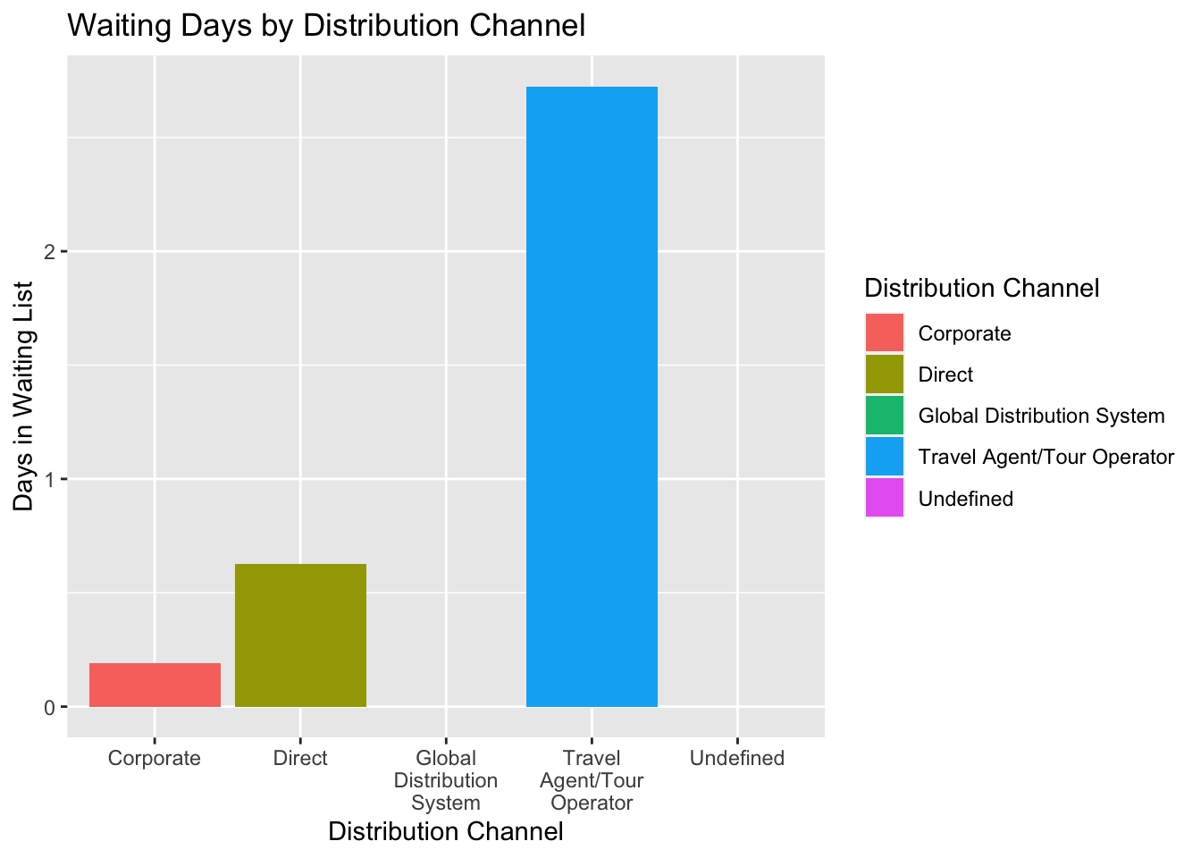
Lastly, I investigate the waiting time associated with different distribution channels. It is evident that bookings made through the Global Distribution System (GDS) exhibit no waiting time. Similarly, Corporate and Direct channels experience minimal waiting periods. In contrast, bookings made through Travel Agents have the longest waiting times. This can be attributed to the fact that Travel Agents rely on GDS or other channels to make bookings, and hotels often prioritize direct or corporate bookings over Travel Agent bookings.
Based on the analysis of market segment and distribution channel in the hotel booking data, we can observe that there is a relationship between these two factors. Different market segments tend to prefer specific distribution channels for making their hotel bookings.
For example, the Travel Agent/Tour Operator distribution channel is popular among customers who prefer booking through Online or Offline Travel Agents. This indicates that targeting these market segments with promotions that highlight the convenience and expertise offered by travel agents could be effective. Additionally, the Group segment shows a significant presence in the Travel Agent/Tour Operator channel, suggesting that promotional efforts can be directed towards attracting group bookings through travel agents.
On the other hand, Direct bookings are favored by individuals who prefer making their reservations directly. To target this segment, promotion strategies can focus on emphasizing the benefits of booking directly, such as greater control, flexibility, and potentially lower costs. Direct booking promotions can highlight features like easy online booking platforms, direct communication with the hotel, and any exclusive benefits or discounts offered to direct bookers.
Considering the different market segments and their preferences, it is important to align the promotional strategies with the specific distribution channels. For instance, promotions targeting the Corporate segment can emphasize the advantages of corporate bookings, such as special rates, dedicated services, and flexible cancellation policies. These promotions can be tailored to reach corporate decision-makers and highlight the benefits of choosing the Corporate channel for their hotel bookings.
Furthermore, based on the analysis of cancellation rates, efforts can be made to reduce cancellations, particularly in the channels with higher cancellation rates. This could include offering incentives or personalized offers to encourage customers to commit to their bookings, implementing flexible booking policies, and improving the overall customer experience to enhance satisfaction and minimize the likelihood of cancellations.
In summary, the analysis of market segment and distribution channel provides insights into customer preferences and behaviors. By aligning promotional strategies with the specific market segments and distribution channels, hotels can effectively target their marketing efforts, tailor their messaging, and optimize their promotional campaigns to attract and retain customers across different channels.
In the process of putting together this project, I have learned several insights about hotel bookings and lead time. Initially, I explored the mean lead time for hotel bookings and discovered that, on average, people tend to book their stays approximately 3 to 3.5 months in advance. This led me to investigate the difference in lead time between Resort hotels and City hotels.
Contrary to expectations, City hotels had a slightly higher lead time than Resort hotels. However, limitations in the dataset’s data distribution between the two hotel types make it difficult to draw definitive conclusions about the relationship between lead time and hotel type. To gain clarity, I created histograms for lead time distributions, allowing for a direct comparison and assessment of central tendencies.
The analysis of the relationship between lead time and the number of children did not reveal a clear pattern. Median lead time varied between 55 and 70 days for people with or without children, suggesting that the presence of children may not strongly influence lead time.
It is important to acknowledge the limitations of the dataset. The uneven distribution of data between hotel types and potential missing variables, such as customer demographics or reasons for travel, limit the depth of analysis. Additionally, the dataset does not capture certain factors that could influence lead time, such as special events, travel restrictions, or seasonal variations.
From the analysis of the cancellation data, several key insights have emerged.The analysis showed no significant cancellation trend based on market segment, but disparities were observed between City hotels and Resort hotels. Bookings without a deposit had higher cancellation rates, including Non Refundable bookings. June had the highest cancellation rate, possibly due to summer vacations, while January had the lowest cancellation rate reflecting winter travel patterns. Longer lead times were associated with higher cancellation rates, particularly for bookings made well in advance.
While these insights shed light on cancellation patterns in hotel bookings, there are still areas to explore. Future research could investigate additional factors influencing cancellations, such as customer demographics, travel purposes, or the presence of specific events or circumstances. This could provide a deeper understanding of the underlying reasons for cancellations and help develop more targeted strategies to mitigate them.
Regarding the limitations of the dataset, it is important to acknowledge several factors. Firstly, the dataset does not capture all the relevant variables that could impact cancellations, such as customer preferences, travel restrictions, or external events. Additionally, the dataset is not representative of the entire hotel industry, as it includes data from specific hotels and regions. The uneven distribution of data between hotel types, market segments, or other variables may also affect the robustness of the analysis.
Furthermore, while the analysis explored various aspects of cancellations, there are still questions that the dataset cannot answer. For example, it does not provide insights into the specific reasons behind cancellations, customer satisfaction levels, or the impact of hotel policies on cancellation behavior. These aspects would require additional data or a more targeted research approach.
Through the analysis of market segment and distribution channel in hotel bookings, we learned that different market segments prefer specific distribution channels. This information can guide targeted promotional strategies to attract and retain customers. For example, the Travel Agent/Tour Operator channel is popular among customers who value convenience, while Direct bookings appeal to those seeking control. However, further research is needed to understand customer preferences within each channel and improve promotional efforts. It’s important to acknowledge limitations such as missing factors and the dataset’s focus. Overall, aligning promotions with customer preferences is crucial, and future research can explore additional dimensions of the booking process to enhance marketing strategies.
It is important to acknowledge the limitations of the dataset. The dataset does not capture certain factors that influence customer decision-making, such as individual preferences, personal circumstances, or external factors. Furthermore, the dataset’s focus on market segment and distribution channel does not provide a comprehensive understanding of the entire booking process or the complete customer journey. Therefore, additional data sources and research methods may be required to explore other aspects of hotel bookings, such as pricing strategies, customer reviews, or marketing effectiveness.