Code
library(tidyverse)
knitr::opts_chunk$set(echo = TRUE, warning=FALSE, message=FALSE)library(tidyverse)
knitr::opts_chunk$set(echo = TRUE, warning=FALSE, message=FALSE)The emphasis in this final project is on exploratory data analysis using both graphics and statistics. The dataset used for this final project is the hotel_bookings.csv (https://www.kaggle.com/datasets/jessemostipak/hotel-booking-demand) which is a popular advanced dataset used for exploratory data analysis. This data set contains booking information for a city hotel and a resort hotel, and includes information such as when the booking was made, length of stay, the number of adults, children, and/or babies, the number of available parking spaces, among other things. Also, the data for this dataset is originally from the article Hotel Booking Demand Datasets, written by Nuno Antonio, Ana Almeida, and Luis Nunes for Data in Brief, Volume 22, February 2019.
Hotel reservation cancellations are unavoidable but one of the major challenges in the hotel industry is to avoid cancellation in order to boost a hotel’s revenue and profit margins. Throughout the next few section, we will look at the descriptive statistics, univariate analysis and then then move onto to bivariate analysis where we will take a closer look at the cancellation rate. We will try to determine what are the cancellation rates for the different hotel types, cancellation rate vs. lead time, cancellation rate time trend and a lot of the other variables given in this dataset. Knowing how to predict demand accurately is incredibly important for the hotel industry and if we can get useful insights from the booking data then we can make those canceled rooms available for walk-ins or last minute bookings thus increasing the revenue.
I am going to use the hotel_bookings.csv data set that is already provided to us in the _data folder. This data set is challenging since it is a large data set with 119390 rows and 32 columns and has difficulty rating of 4-star.
data_hotels <- read_csv("_data/hotel_bookings.csv")
data_hotelsglimpse(data_hotels)Rows: 119,390
Columns: 32
$ hotel <chr> "Resort Hotel", "Resort Hotel", "Resort…
$ is_canceled <dbl> 0, 0, 0, 0, 0, 0, 0, 0, 1, 1, 1, 0, 0, …
$ lead_time <dbl> 342, 737, 7, 13, 14, 14, 0, 9, 85, 75, …
$ arrival_date_year <dbl> 2015, 2015, 2015, 2015, 2015, 2015, 201…
$ arrival_date_month <chr> "July", "July", "July", "July", "July",…
$ arrival_date_week_number <dbl> 27, 27, 27, 27, 27, 27, 27, 27, 27, 27,…
$ arrival_date_day_of_month <dbl> 1, 1, 1, 1, 1, 1, 1, 1, 1, 1, 1, 1, 1, …
$ stays_in_weekend_nights <dbl> 0, 0, 0, 0, 0, 0, 0, 0, 0, 0, 0, 0, 0, …
$ stays_in_week_nights <dbl> 0, 0, 1, 1, 2, 2, 2, 2, 3, 3, 4, 4, 4, …
$ adults <dbl> 2, 2, 1, 1, 2, 2, 2, 2, 2, 2, 2, 2, 2, …
$ children <dbl> 0, 0, 0, 0, 0, 0, 0, 0, 0, 0, 0, 0, 0, …
$ babies <dbl> 0, 0, 0, 0, 0, 0, 0, 0, 0, 0, 0, 0, 0, …
$ meal <chr> "BB", "BB", "BB", "BB", "BB", "BB", "BB…
$ country <chr> "PRT", "PRT", "GBR", "GBR", "GBR", "GBR…
$ market_segment <chr> "Direct", "Direct", "Direct", "Corporat…
$ distribution_channel <chr> "Direct", "Direct", "Direct", "Corporat…
$ is_repeated_guest <dbl> 0, 0, 0, 0, 0, 0, 0, 0, 0, 0, 0, 0, 0, …
$ previous_cancellations <dbl> 0, 0, 0, 0, 0, 0, 0, 0, 0, 0, 0, 0, 0, …
$ previous_bookings_not_canceled <dbl> 0, 0, 0, 0, 0, 0, 0, 0, 0, 0, 0, 0, 0, …
$ reserved_room_type <chr> "C", "C", "A", "A", "A", "A", "C", "C",…
$ assigned_room_type <chr> "C", "C", "C", "A", "A", "A", "C", "C",…
$ booking_changes <dbl> 3, 4, 0, 0, 0, 0, 0, 0, 0, 0, 0, 0, 0, …
$ deposit_type <chr> "No Deposit", "No Deposit", "No Deposit…
$ agent <chr> "NULL", "NULL", "NULL", "304", "240", "…
$ company <chr> "NULL", "NULL", "NULL", "NULL", "NULL",…
$ days_in_waiting_list <dbl> 0, 0, 0, 0, 0, 0, 0, 0, 0, 0, 0, 0, 0, …
$ customer_type <chr> "Transient", "Transient", "Transient", …
$ adr <dbl> 0.00, 0.00, 75.00, 75.00, 98.00, 98.00,…
$ required_car_parking_spaces <dbl> 0, 0, 0, 0, 0, 0, 0, 0, 0, 0, 0, 0, 0, …
$ total_of_special_requests <dbl> 0, 0, 0, 0, 1, 1, 0, 1, 1, 0, 0, 0, 3, …
$ reservation_status <chr> "Check-Out", "Check-Out", "Check-Out", …
$ reservation_status_date <date> 2015-07-01, 2015-07-01, 2015-07-02, 20…Ans: The code for cleaning the hotel_booking data set is given below:
colSums(is.na(data_hotels)) hotel is_canceled
0 0
lead_time arrival_date_year
0 0
arrival_date_month arrival_date_week_number
0 0
arrival_date_day_of_month stays_in_weekend_nights
0 0
stays_in_week_nights adults
0 0
children babies
4 0
meal country
0 0
market_segment distribution_channel
0 0
is_repeated_guest previous_cancellations
0 0
previous_bookings_not_canceled reserved_room_type
0 0
assigned_room_type booking_changes
0 0
deposit_type agent
0 0
company days_in_waiting_list
0 0
customer_type adr
0 0
required_car_parking_spaces total_of_special_requests
0 0
reservation_status reservation_status_date
0 0 Also there are a few rows in the data set where no adult or there are children with no adults that have checked in. Now babies and children can’t check-in on their own so we will remove those entries from the data set.
data_hotels <- data_hotels %>% filter(data_hotels$adults != 0)This concludes the data cleaning for the final project. In the next few sections, we will go in depth about some of the descriptive statistics about the dataset.
Ans: After cleaning the data set above we can now see that it has 118,987 rows and 32 columns.
glimpse(data_hotels)Rows: 118,987
Columns: 32
$ hotel <chr> "Resort Hotel", "Resort Hotel", "Resort…
$ is_canceled <dbl> 0, 0, 0, 0, 0, 0, 0, 0, 1, 1, 1, 0, 0, …
$ lead_time <dbl> 342, 737, 7, 13, 14, 14, 0, 9, 85, 75, …
$ arrival_date_year <dbl> 2015, 2015, 2015, 2015, 2015, 2015, 201…
$ arrival_date_month <chr> "July", "July", "July", "July", "July",…
$ arrival_date_week_number <dbl> 27, 27, 27, 27, 27, 27, 27, 27, 27, 27,…
$ arrival_date_day_of_month <dbl> 1, 1, 1, 1, 1, 1, 1, 1, 1, 1, 1, 1, 1, …
$ stays_in_weekend_nights <dbl> 0, 0, 0, 0, 0, 0, 0, 0, 0, 0, 0, 0, 0, …
$ stays_in_week_nights <dbl> 0, 0, 1, 1, 2, 2, 2, 2, 3, 3, 4, 4, 4, …
$ adults <dbl> 2, 2, 1, 1, 2, 2, 2, 2, 2, 2, 2, 2, 2, …
$ children <dbl> 0, 0, 0, 0, 0, 0, 0, 0, 0, 0, 0, 0, 0, …
$ babies <dbl> 0, 0, 0, 0, 0, 0, 0, 0, 0, 0, 0, 0, 0, …
$ meal <chr> "BB", "BB", "BB", "BB", "BB", "BB", "BB…
$ country <chr> "PRT", "PRT", "GBR", "GBR", "GBR", "GBR…
$ market_segment <chr> "Direct", "Direct", "Direct", "Corporat…
$ distribution_channel <chr> "Direct", "Direct", "Direct", "Corporat…
$ is_repeated_guest <dbl> 0, 0, 0, 0, 0, 0, 0, 0, 0, 0, 0, 0, 0, …
$ previous_cancellations <dbl> 0, 0, 0, 0, 0, 0, 0, 0, 0, 0, 0, 0, 0, …
$ previous_bookings_not_canceled <dbl> 0, 0, 0, 0, 0, 0, 0, 0, 0, 0, 0, 0, 0, …
$ reserved_room_type <chr> "C", "C", "A", "A", "A", "A", "C", "C",…
$ assigned_room_type <chr> "C", "C", "C", "A", "A", "A", "C", "C",…
$ booking_changes <dbl> 3, 4, 0, 0, 0, 0, 0, 0, 0, 0, 0, 0, 0, …
$ deposit_type <chr> "No Deposit", "No Deposit", "No Deposit…
$ agent <chr> "NULL", "NULL", "NULL", "304", "240", "…
$ company <chr> "NULL", "NULL", "NULL", "NULL", "NULL",…
$ days_in_waiting_list <dbl> 0, 0, 0, 0, 0, 0, 0, 0, 0, 0, 0, 0, 0, …
$ customer_type <chr> "Transient", "Transient", "Transient", …
$ adr <dbl> 0.00, 0.00, 75.00, 75.00, 98.00, 98.00,…
$ required_car_parking_spaces <dbl> 0, 0, 0, 0, 0, 0, 0, 0, 0, 0, 0, 0, 0, …
$ total_of_special_requests <dbl> 0, 0, 0, 0, 1, 1, 0, 1, 1, 0, 0, 0, 3, …
$ reservation_status <chr> "Check-Out", "Check-Out", "Check-Out", …
$ reservation_status_date <date> 2015-07-01, 2015-07-01, 2015-07-02, 20…The descriptive statistics help us give some background information about the dataset. For the sake of simplicity, I have only provided the descriptive statistics for a few of the variables in our dataset. There are 32 columns (variables) and hence it would be very difficult to provide information for each and every variable. In the section given below, I have provided the descriptive statistics for a few of the important variables. There are a few important variables that are skipped in this section but they will be separately covered in the research question section.
Firstly, the exhaustive table of the mean, median and standard deviation for all the variables is given in the summary dataframe below. Some important statistics that we can see from the table below is that the lead_time_mean is 104.07, adults_median staying is 2, the mean of the Average Daily Rate($) is 102.01, and the median of the Average Daily Rate is 95.
summary <- data_hotels %>% summarize(across(everything(), list(mean = mean, median = median, sd = sd), na.rm = TRUE))

summary
For the categorical variables, we can find the frequency table to get a better idea of their distribution.
To start off with the categorical variables, we can look at the number of reservations that are successfully checked-out vs canceled vs No-show. Observing the data, we can say that a significant chunk of the reservations are checked out followed by canceled. No-show only accounts for a small fraction of the total reservations.
df1<- as_tibble(as.data.frame(table(data_hotels$reservation_status)))
df1df1$Percentage <- df1$Freq / sum(df1$Freq)
df1$Label <- paste0(df1$Var1, " (", scales::percent(df1$Percentage), ")")
# Create the pie chart
pie_reservation <- ggplot(df1, aes(x = "", y = Percentage, fill = Label)) +
geom_bar(width = 1, stat = "identity") +
coord_polar("y", start = 0) +
theme_void() +
theme(legend.position = "right") +
labs(x = NULL, y = NULL, fill = NULL,
title = "Pie Chart of Reservation Status for Hotel Bookings")
pie_reservation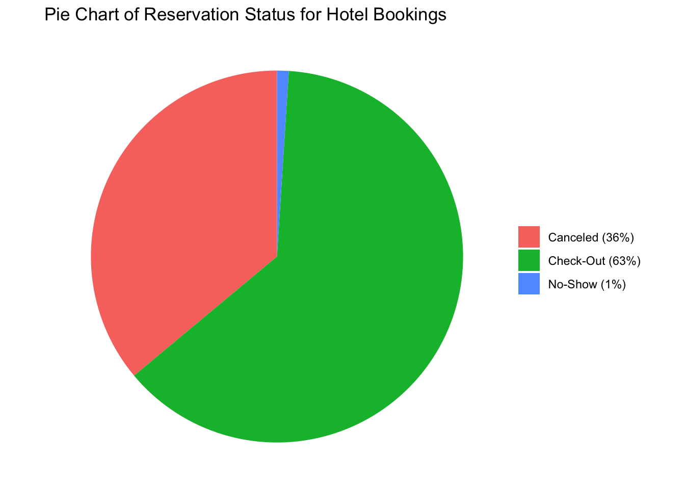
Similarly, we can analyze the meal type by creating a table and plotting a bar chart. Out of the meals, BB (Bed & Breakfast) is the most ordered meal which is around 77.3%, followed by HB(Half Board), SC(no meal package), Undefined and FB (Full Board).
table(data_hotels$meal)
       BB        FB        HB        SC Undefined
92020 798 14454 10546 1169 prop.table(table(data_hotels$meal))
         BB          FB          HB          SC   Undefined
0.773361796 0.006706615 0.121475455 0.088631531 0.009824603 sum_table_0 <- data_hotels %>%
group_by(meal) %>%
summarize(count = n(), .groups='drop') %>% arrange(desc(count))
ggplot(sum_table_0, aes(x=reorder(meal,desc(count)), y=count)) + geom_bar(stat = "identity", fill = "maroon")+labs(x = "Meal Type", y = "Count", title = "Bar Chart of Count vs Meal Type") + theme(axis.text.x = element_text(angle = 90, vjust = 0.5, hjust=1)) 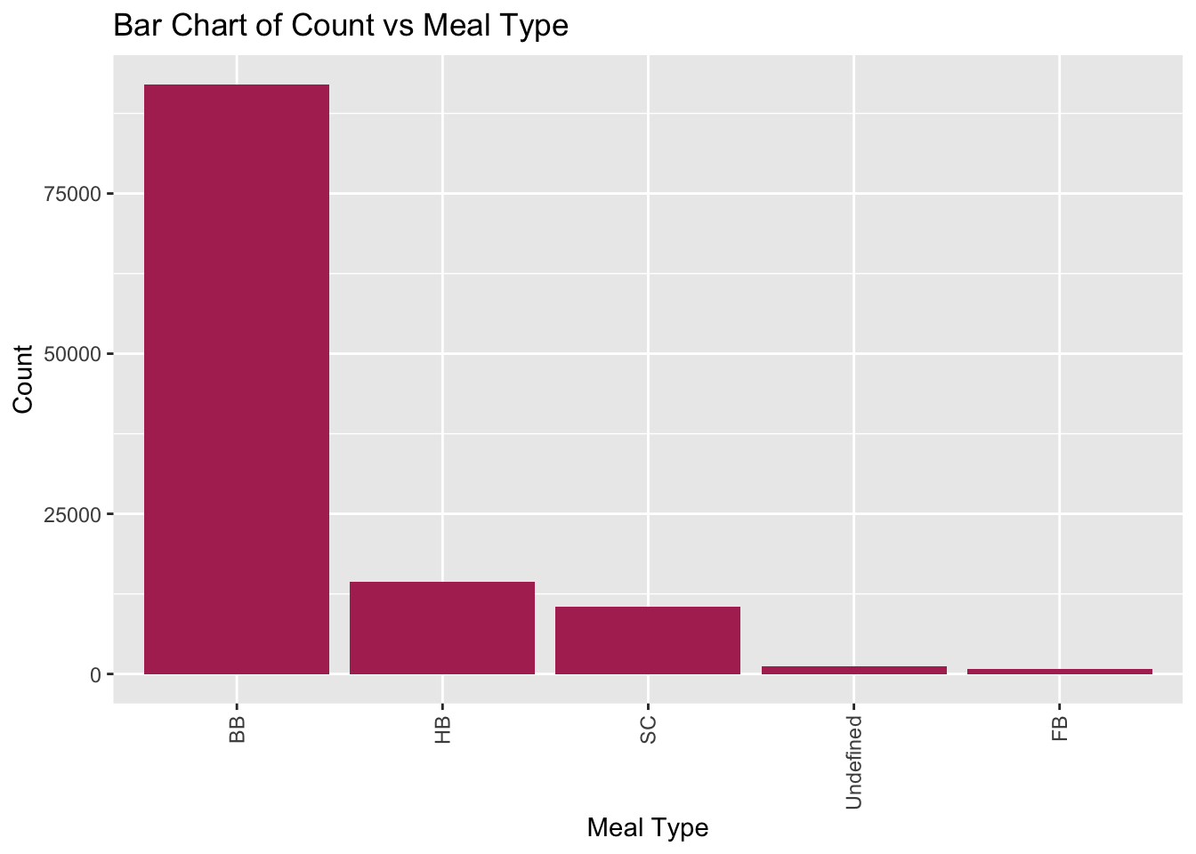
Next, we look at the market segment which is responsible for the hotel bookings. I have restructured the table to be converted into a tibble, so that it can be used to plot the pie chart given below.
df<- as_tibble(as.data.frame(table(data_hotels$market_segment)))
df
From the pie chart below, we can conclude that roughly half (47.25%) of all the hotel bookings are done via the online TA (Travel Agent). This includes websites like Expedia, and hotels.com. The next major segment is the offline TA (20.32%), which may include bookings done by a human travel agent or in-person bookings. Aviation, Complementary, Corporate, Direct and Groups together contribute to around 1/3 of the total market share.
df$Percentage <- df$Freq / sum(df$Freq)
df$Label <- paste0(df$Var1, " (", scales::percent(df$Percentage), ")")

# Create the pie chart
pie<- ggplot(df, aes(x = "", y = Percentage, fill = Label)) +
  geom_bar(width = 1, stat = "identity") +
  coord_polar("y", start = 0) +
  theme_void() +
  theme(legend.position = "right") +
  labs(x = NULL, y = NULL, fill = NULL,
       title = "Pie Chart of Market Segment for Hotel Bookings")

pie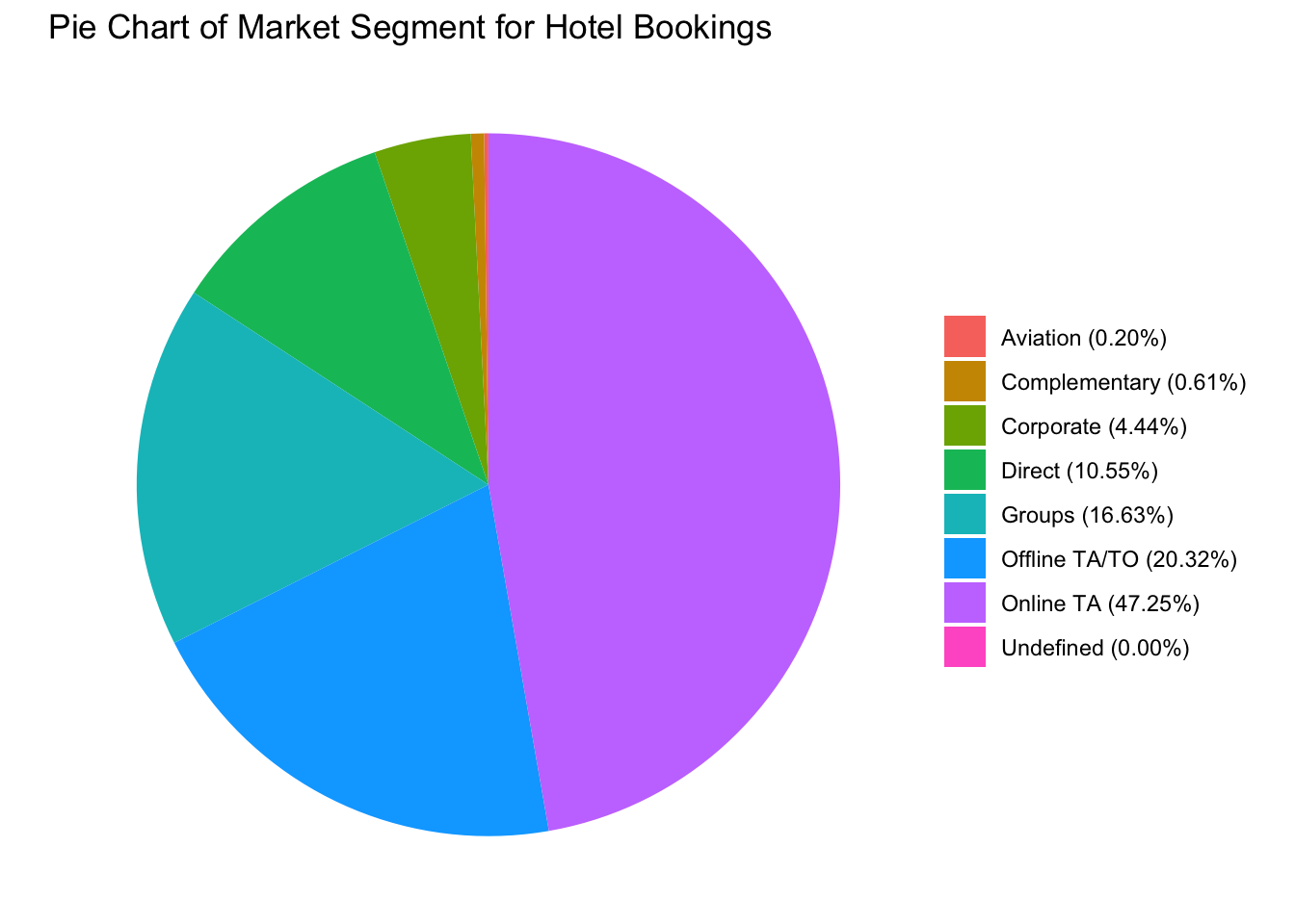
Looking at yet another categorical variable, we can see that the most popular room type among guests is type A. The next in order is type D, E, F. One important point to note is that the room type A is popular compared to the next few room types by a significant margin. In fact, the number of bookings for room type A are greater than the sum of all the other room types combined.
table(data_hotels$assigned_room_type)
    A     B     C     D     E     F     G     H     I     K     L
73983 1972 2370 25306 7798 3751 2548 712 359 187 1 sum_table_1 <- data_hotels %>%
group_by(assigned_room_type) %>%
summarize(count = n(), .groups='drop') %>% arrange(desc(count))
ggplot(sum_table_1, aes(x=reorder(assigned_room_type,desc(count)), y=count)) + geom_bar(stat = "identity",fill = "darkgreen")+labs(x = "Assigned Room Type", y = "Count", title = "Bar Chart of Count vs Assigned Room Type") +theme(axis.text.x = element_text(angle = 90, vjust = 0.5, hjust=1))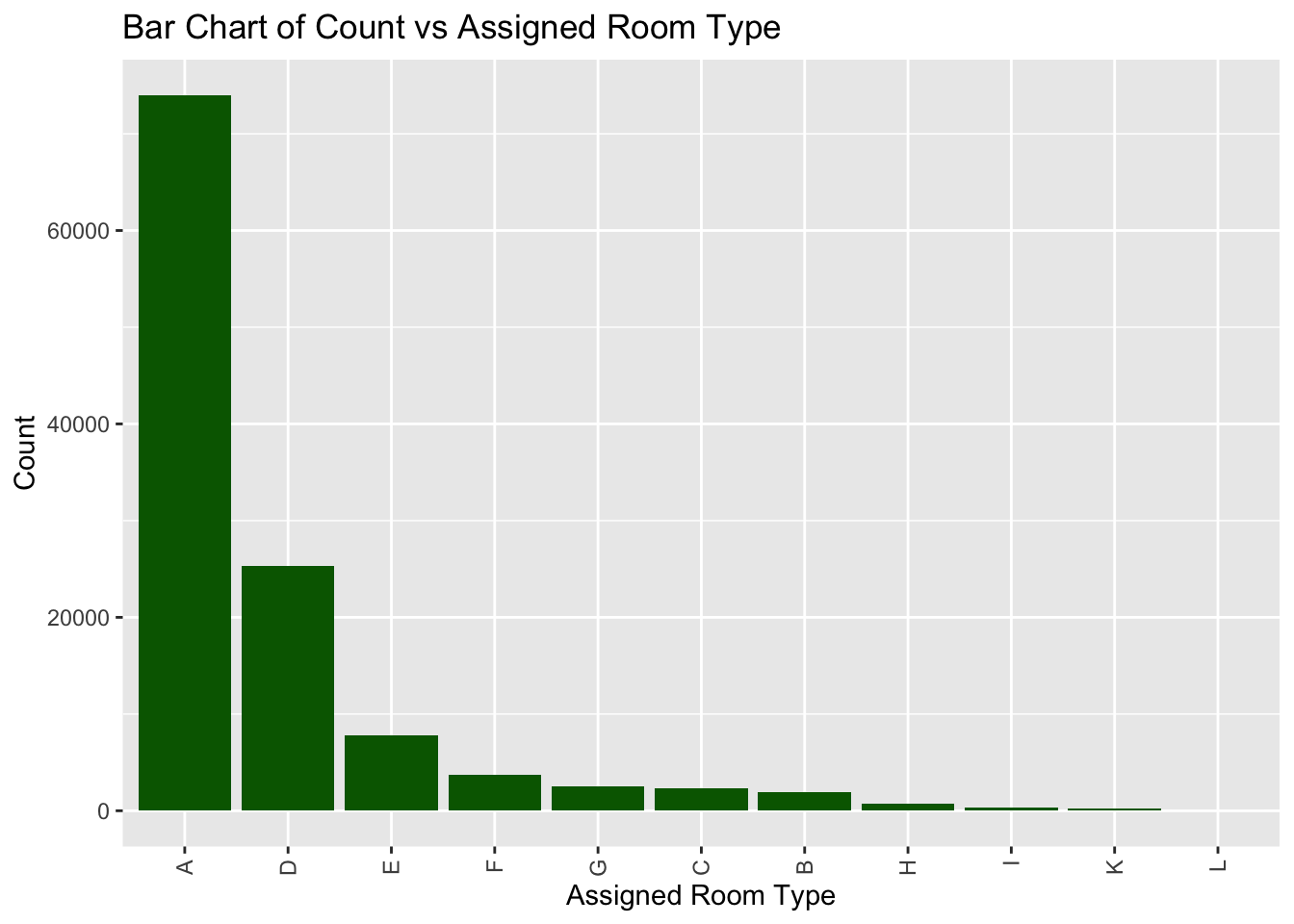
Shown below, is the pareto bar chart for the customer type variable. As we can see, the majority of the customers (>75%) are of the ‘Transient’ type. The next biggest customer group is the Transient
table(data_hotels$customer_type)
       Contract           Group       Transient Transient-Party
4071 573 89337 25006 prop.table(table(data_hotels$customer_type))
       Contract           Group       Transient Transient-Party
0.034213822 0.004815652 0.750813114 0.210157412 sum_table_2 <- data_hotels %>%
group_by(customer_type) %>%
summarize(count = n(), .groups='drop') %>% arrange(desc(count))
ggplot(sum_table_2, aes(x=reorder(customer_type,desc(count)), y=count)) + geom_bar(stat = "identity",fill = "purple") + labs(x = "Customer Type", y = "Count", title = "Bar Chart of Count vs Customer Type") +theme(axis.text.x = element_text(angle = 90, vjust = 0.5, hjust=1))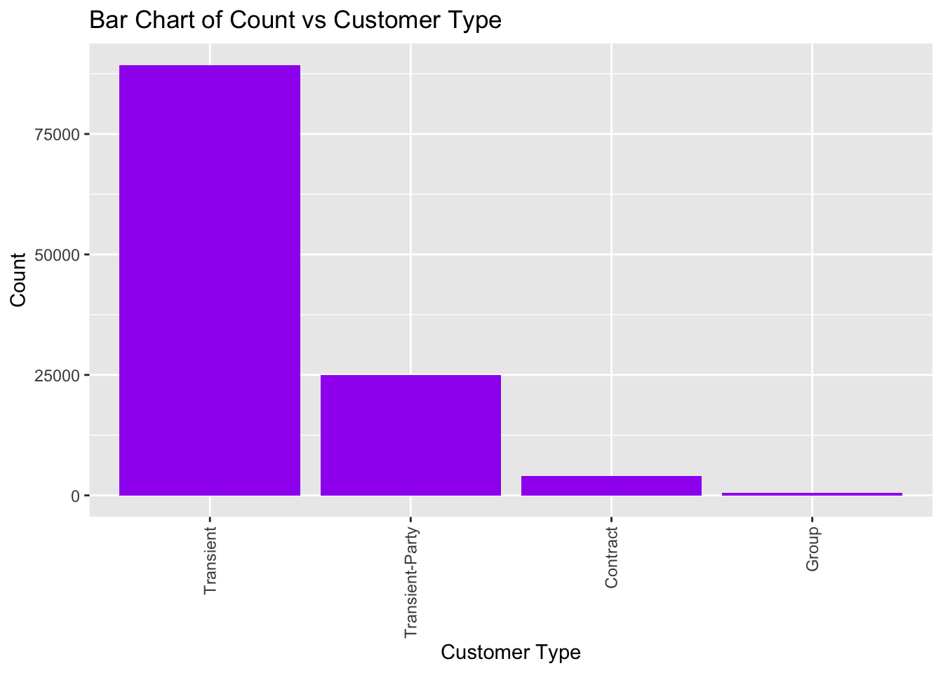
Lastly, the histogram plot below shows the average daily rate (in $) for all the different hotels faceted by the hotel type. Looking at the density plot below, we can conclude that the city hotels have a bimodal distribution around 60-100 USD. This means that there are some cheaper hotels that are for 60, but there are a few expensive ones that rent for 100 USD. On the other hand, for resort hotels the distribution is much more smooth with a maximum density around 50 USD. From this we can conclude that, on an average, city hotels are more expensive to rent as compared to resort style hotels. This makes sense since resort hotels are usually located on the outskirts of a city where the land is cheaper and there is more space to build a large resort style hotel. City hotels, on the other hand, are built in/near the city downtown where the real estate is much more expensive.
ggplot(data_hotels, aes(adr)) +
  geom_histogram(aes(y = ..density..), alpha = 0.7) +
  geom_density(alpha = 0.2, fill="red") + xlim(0,300) +labs(x="Average Daily Rate($)",y="Density",title="Histogram Density of Average Daily Rate(ADR)") + facet_wrap(~hotel)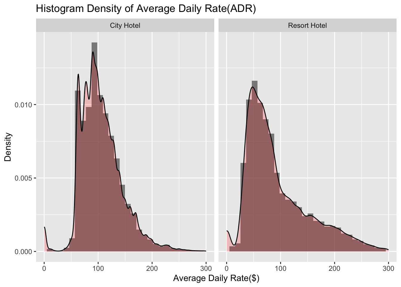
What is the preferred hotel type for guests (City hotel vs Resort hotel)?
Hotel bookings are usually seasonal in nature. Which month has the highest number of bookings?
Which countries have the highest number of incoming guests?
What is the average length of stay per booking? Average number of guests per booking?
How does the ADR (Average Daily Rate) vary with the lead time?
Does the ADR (Average Daily Rate) change with the day of the month?
How does the number of cancellations change with the customer type?
Which months have the highest number of cancellations?
How does the cancellation fraction change with the deposit type? I.e. are refundable deposit bookings more likely to be canceled?
How does the cancellation fraction change with the market segment?
Does longer lead time result in higher number of cancellations?
We can see that there are two different types of hotels; Resort hotels and City hotels. The number of City Hotels accounts for 66.3% of the total hotels in this dataset. Resort hotels account for 33.65% of the total hotel bookings. Hence there are almost twice as many City Hotel booking as there are Resort Hotel bookings. From that we can infer that guests prefer City Hotels much more than Resort style hotels.
table(data_hotels$hotel)
  City Hotel Resort Hotel
78940 40047 prop.table(table(data_hotels$hotel))
  City Hotel Resort Hotel
0.6634338 0.3365662 ggplot(data_hotels, aes(hotel)) + geom_bar(fill = "navyblue")+labs(x = "Hotel Type", y = "Number of Bookings", title = "Bar Chart of Count vs Hotel Type") +theme(axis.text.x = element_text(angle = 90, vjust = 0.5, hjust=1))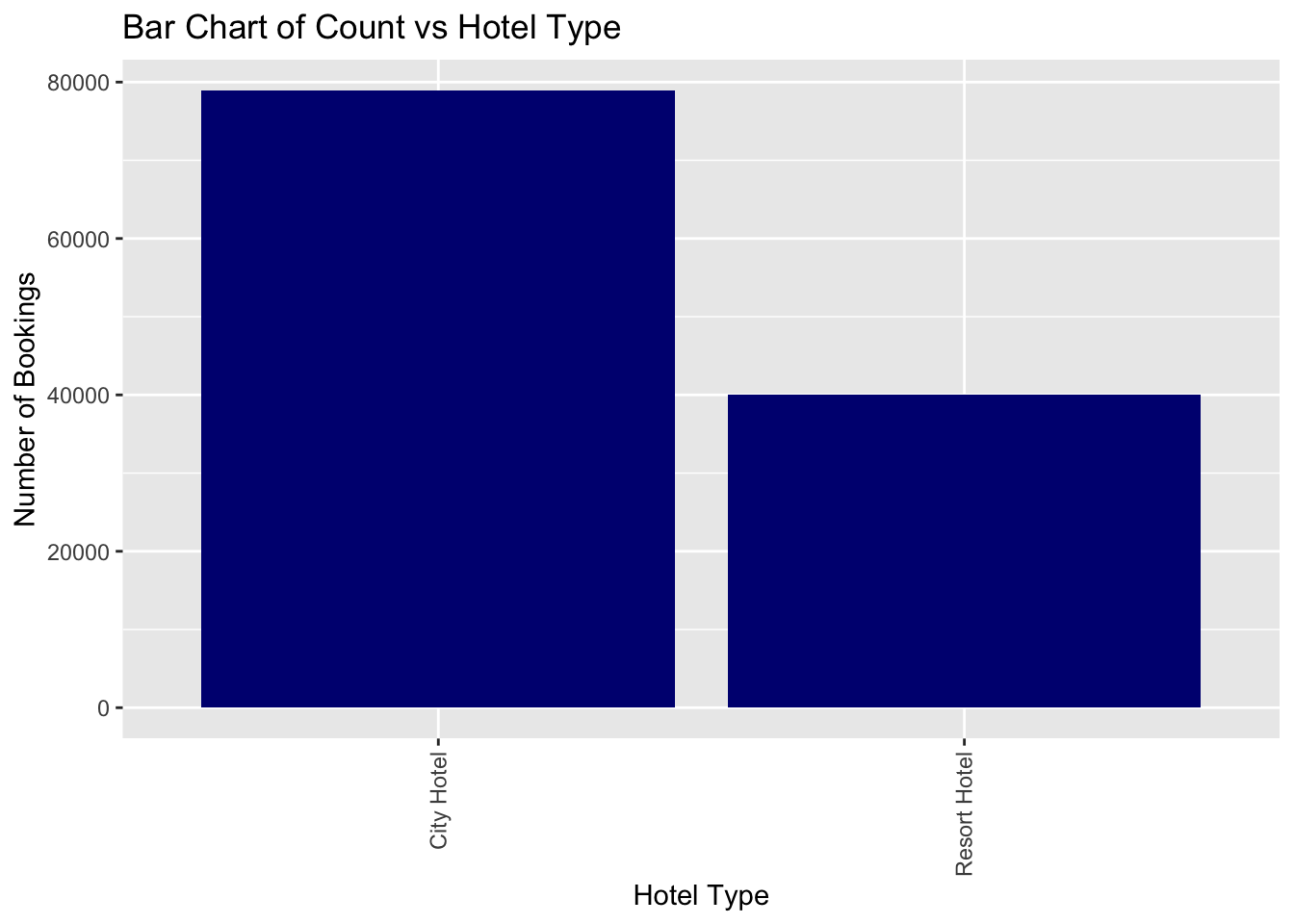
Hence the City Hotel is much more preferable for the guests as compared to Resort Hotels.
It is a well known phenomena that hotel bookings are seasonal in nature. The data provided to us will help reaffirm the notion. Post the data cleaning performed in the ‘Data Cleaning’ section, we can see that there is some data missing for the 2015 and 2017. This might likely be due to the fact that someone(clerk, manager) erroneously entered the wrong data for those months and it was filtered out(adults != 0) when we performed the data cleaning. But based on the available data, we can see from the plot given below that the number of bookings usually starts out high in Jan and Feb and gradually goes down till May. This makes sense since the start of the year a lot of people have holidays and are recovering from the end of the year vacations. March and April are usually not holiday seasons and hence the total number of bookings is low. But there is a sudden surge in bookings after June, all the way through July.
This increase in the number of bookings is due to the summer vacations. A lot of families and students usually take atleast a week off for summer break. The booking rate then decreases after summer till we reach the end of the year. The number of bookings increases in November and December since people are celebrating their Christmas holidays. Thus, we are able to get a good picture of the overall seasonal trend in the hotel bookings from the plot given below.
data_hotels %>% ggplot(aes(x=arrival_date_month, fill=hotel)) +
  geom_bar(position="dodge") +
  scale_fill_manual(values=c("azure4", "azure3"),labels=c("City Hotel", "Resort Hotel")) +
  scale_y_continuous(name = "Bookings",labels = scales::comma) +
  guides(fill=guide_legend(title=NULL))  +
  facet_grid(arrival_date_year ~ .) +
  theme(legend.position="bottom", axis.text.x=element_text(angle=0, hjust=1, vjust=0.5)) +
scale_x_discrete(labels=c("Jan","Feb","Mar","Apr","May","Jun","Jul","Aug","Sep","Oct","Nov","Dec" )) + labs(x="", y="Bookings",title="Number of Bookings vs. Time (in Months)", subtitle="Faceted by year") 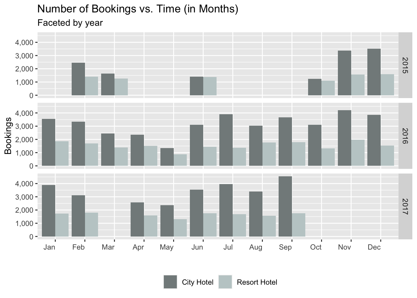
We can also get an idea of the nationality of the different guest by looking at the list of countries below:
data_hotels %>%
  group_by(country)%>%
  summarise(num=n())%>%
  arrange(desc(num))
Based on the data above of the top 15 countries (arranged in desc order), the top 3 countries are Portugal(PRT), Great Britain(GBR) and France (FRA).
This is visualized in the plot given below:
data_country <- data_hotels %>% group_by(country) %>%  summarise(booking_count = n()) %>% arrange(desc(booking_count))
top_n(data_country,15,booking_count) %>%
  ggplot(aes(x = reorder(country,booking_count), y = booking_count)) +
  geom_bar(stat = "identity", width = 0.25, fill="navyblue")+
 coord_flip()+
   ylab('Number of Bookings')+
  xlab('Nationality')+
  ggtitle('Number of Bookings by Country') +
  labs(fill='Hotel type')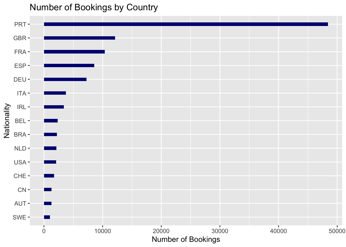
From the plot given below and the data summary, we can see that the median length of stay per booking is 3 days. The mean is 3.45 days.
weekend<-data_hotels$stays_in_weekend_nights
week<-data_hotels$stays_in_week_nights
total<-weekend+week
total[total==0]<-NA
summary(total)
Min. 1st Qu. Median Mean 3rd Qu. Max. NA's
1.000 2.000 3.000 3.445 4.000 69.000 645 ggplot(data_hotels, aes(total)) +
geom_histogram(fill="brown",bins = 30) + labs(title = "Length of Stay", x = "Number of Days", y = "Count") + xlim(0,30)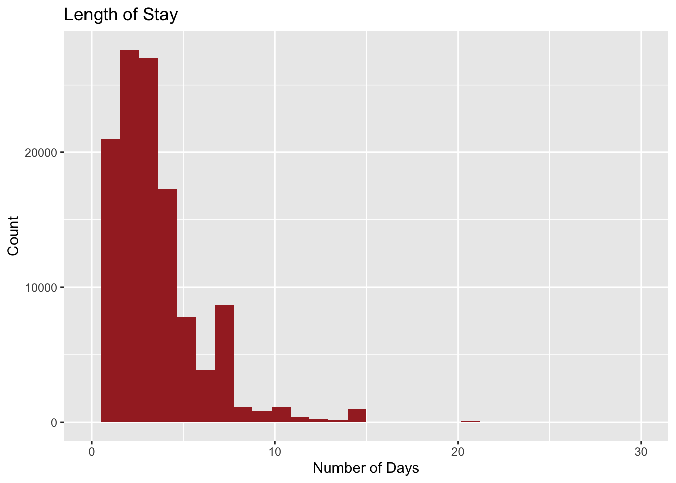
Also, the average number of guests per booking is 2. This is includes all three categories; adults, babies and children.
num_guests<-data_hotels$adults + data_hotels$children + data_hotels$babies

num_guests[num_guests==0]<-NA
summary(num_guests)
Min. 1st Qu. Median Mean 3rd Qu. Max. NA's
1.000 2.000 2.000 1.971 2.000 55.000 4 ggplot(data_hotels, aes(num_guests)) +
geom_histogram(fill = 'darkgreen',bins = 30) + labs(title = "Average Number of Guests", subtitle="Includes children and babies", x = "Number of Guests", y = "Count") + xlim(0,6)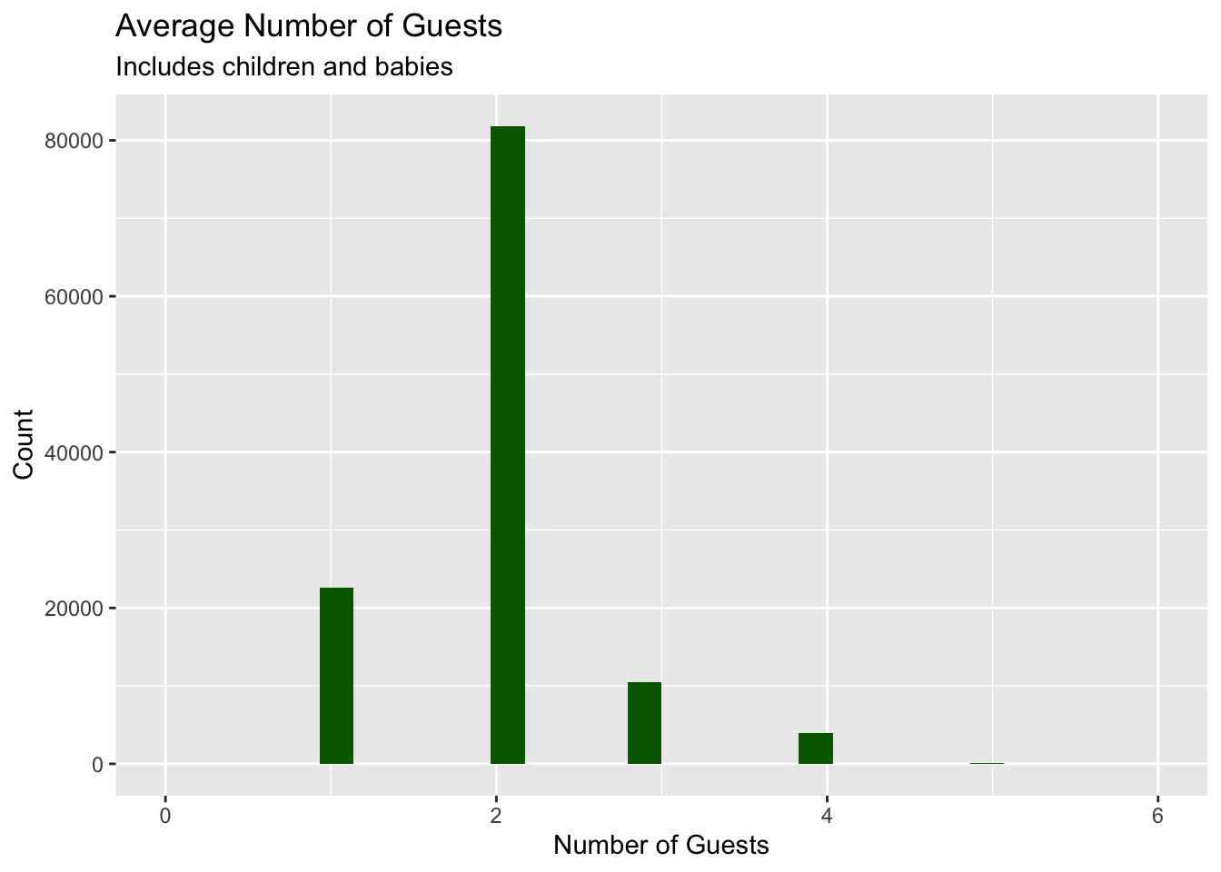
The main question that is being asked here is whether it is cheaper to rent a hotel room if it is booked in advance. The lead time is the number of days the booking was done prior to the date of arrival. From the plot given below we can see the relation between the Average Daily Rate(ADR in $) and lead_time faceted by the hotel type. There is a large density around the range of 0-30 days but then it scatters out as the lead time increases. Also resort hotels have a lower average price as compare to city hotels and prices drop significantly more for resort hotels than city hotels as the lead_time increases.
Hence to achieve a lower price when booking a resort hotel, one can generally book ahead of time for just a bit more days (~ 20-30 days) to watch for the price to drop. This is better than waiting for the price to drop for city hotel because city hotel generally takes longer lead_time (around 60 days) to have a big variance in the ADR as per the dataset. Therefore, using our dataset we have proven that indeed it is cheaper to rent a hotel room if it is booked in advance but it is more prevalent for resort hotels than city hotels.
ggplot(data_hotels, aes(lead_time, adr)) + geom_point(alpha=0.01) +
labs(title = "Average Daily Rate (ADR) vs lead_time", subtitle ="Faceted by Hotel Type", x="lead_time (in days)",y="Average Daily Rate (ADR in $)") + ylim(0,300) + facet_wrap(~hotel)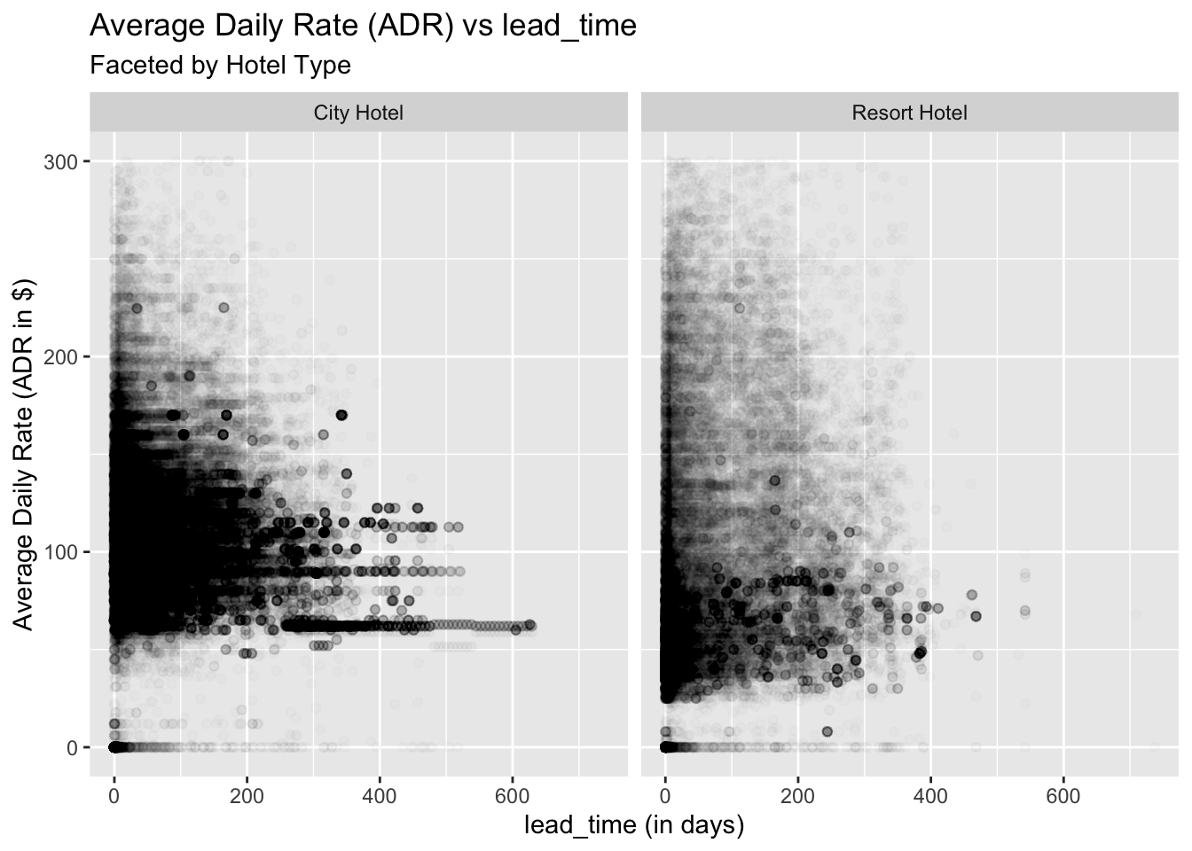
The main question that is being asked here is whether it is cheaper to book a room on certain dates in a month. From the plot given below, we can see that there is very little variability for city hotels. On the other hand, for resort hotels, we do see some increase in ADR during the start(1st) and end of the month (30th-31st). We can explain this behavior by understanding the nature of travelers visiting both the hotels. For city hotels, the visitors are mostly businessmen or professionals attending a conference or tourist who are visiting the city for sightseeing. Hence there is a constant demand for city hotels which is seen in the almost flat ADR rate. But for resort hotels, the visitors are usually seasonal guests who are on vacation/holiday which is why there is a higher demand (and hence higher ADR) towards the end of the month.
grouped_by_day <- data_hotels %>% mutate(arrival_date_day_of_month=as.character(arrival_date_day_of_month)) %>% group_by(arrival_date_day_of_month)

ggplot(grouped_by_day, aes(x = reorder(arrival_date_day_of_month,as.numeric(arrival_date_day_of_month)), y = adr, fill = hotel)) +
  geom_boxplot() + labs(x = "Day of the Month", y = "Average Daily Rate (ADR in $)") + ylim(0,250) + theme(axis.text.x = element_text(size=4))+ facet_wrap(~hotel)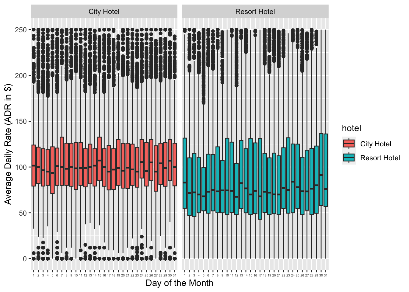
As a hotel owner, knowing the answer to the above question can really help the hotel with customer retention. The main question we are concerned about is, if certain types of customers are more likely to cancel their booking? From the plot given below, we can see that Transient customer (i.e. individual guests not belonging to any group or corporation ) are much more likely to cancel their hotel reservations. Also, looking at the stacked chart below, it is evident that the among Transient customers, city hotels have a higher number of cancellations (~3x) as compared to resort hotels. Hence as a hotel owner, one should make sure to provide complimentary benefits/added incentives for Transient guests so that they do not cancel their bookings.
canceled_bookings_guest <- data_hotels %>% select(hotel,is_canceled,customer_type) %>% filter(is_canceled == 1) %>% group_by(customer_type,hotel) %>% summarise(count = n()) %>% arrange(desc(count))
canceled_bookings_guestggplot(canceled_bookings_guest,aes(x = reorder(customer_type,count), y = count,fill=hotel)) + geom_bar(position="stack", stat="identity") + coord_flip() + labs(title='Number of Cancellations vs. Customer Type',x="Customer Type",y="Number of Cancellations")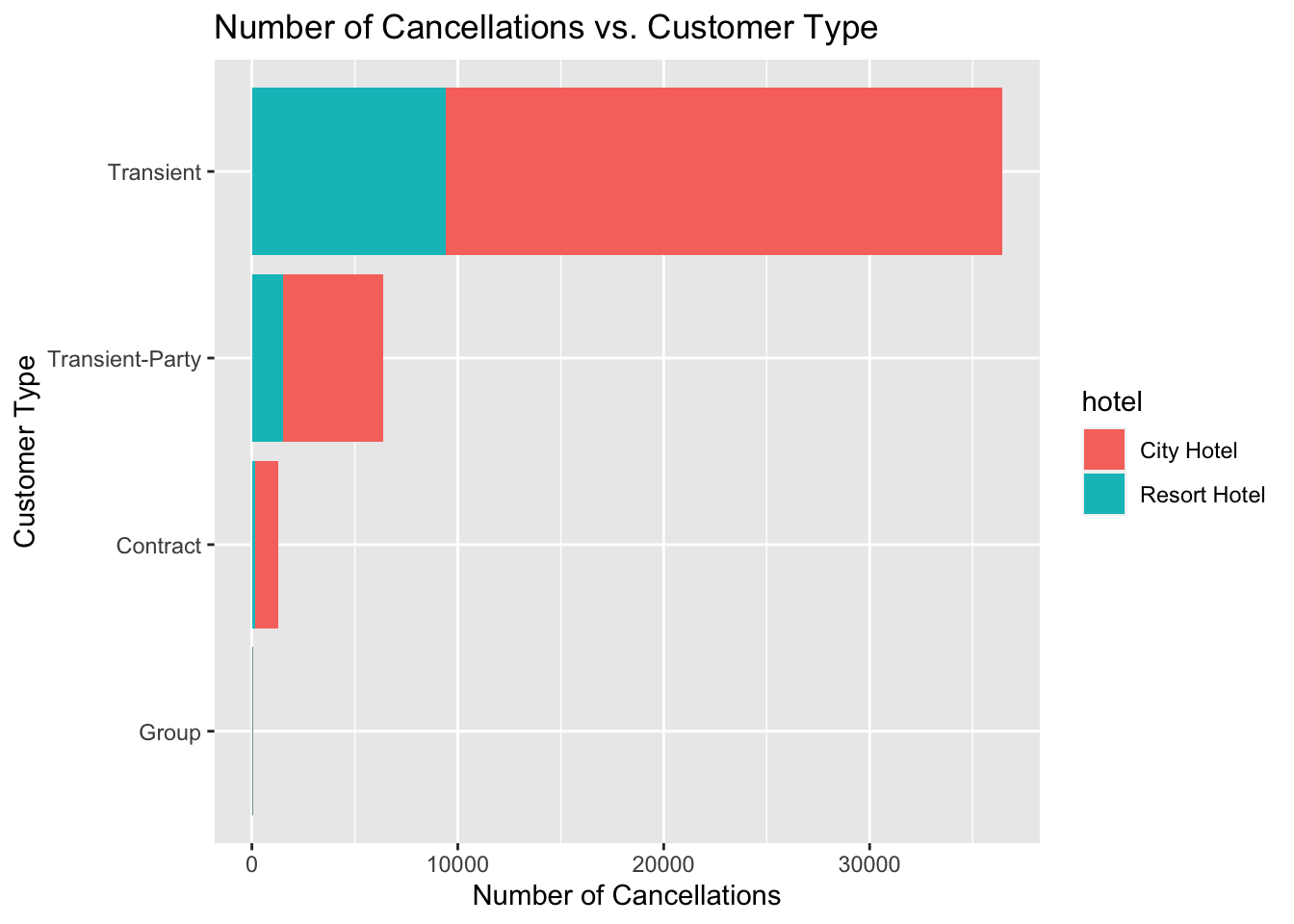
From the Univariate Research Question #2, we know that the number of booking is seasonal in nature. But are the number of cancellations also seasonal? Lets look at the plot below. The missing data for the months in 2015 and 2017 is likely due to the data cleaning performed on the data. But the plot given below shows a similar trend to the plot in URQ#2. There are a high number of cancellations at the start of the year in Jan for both hotel types. This rate drops till it reaches Jun and then it spikes back up in July. Since there a lot of travelers in the summer holiday season, a lot of people miss their flights/trains, and hence we see an increase in the cancellations during summer. The cancellations stays almost steady for the next few months until we reach the end of the year. The cancellation rate then spikes up in Nov and Dec as we enter the Christmas holiday season. There are a lot of travelers in November and December as well and since there are numerous cancellation due to delayed flights/inclement snowy weather, we see a spike in the total number of cancellations. Thus the number of cancellations are also seasonal in nature.
canceled_bookings <- data_hotels %>% select(hotel,is_canceled,arrival_date_year,arrival_date_month) %>% filter(is_canceled == 1)

canceled_bookings %>% ggplot(aes(x=arrival_date_month, fill=hotel)) +
  geom_bar(position="dodge") +
  scale_fill_manual(values=c("blue", "navyblue"),labels=c("City Hotel", "Resort Hotel")) +
  scale_y_continuous(name = "Number of Cancellations (is_canceled)",labels = scales::comma) +
  guides(fill=guide_legend(title=NULL))  +
  facet_grid(arrival_date_year ~ .) +
  theme(legend.position="bottom", axis.text.x=element_text(angle=0, hjust=1, vjust=0.5)) +
scale_x_discrete(labels=c("Jan","Feb","Mar","Apr","May","Jun","Jul","Aug","Sep","Oct","Nov","Dec" )) + labs(x="Time in Months(arrival_time_month)", y="Number of Cancellations (is_canceled)", title="Number of Booking Cancellations vs Time in Months", subtitle = "Faceted by Year") 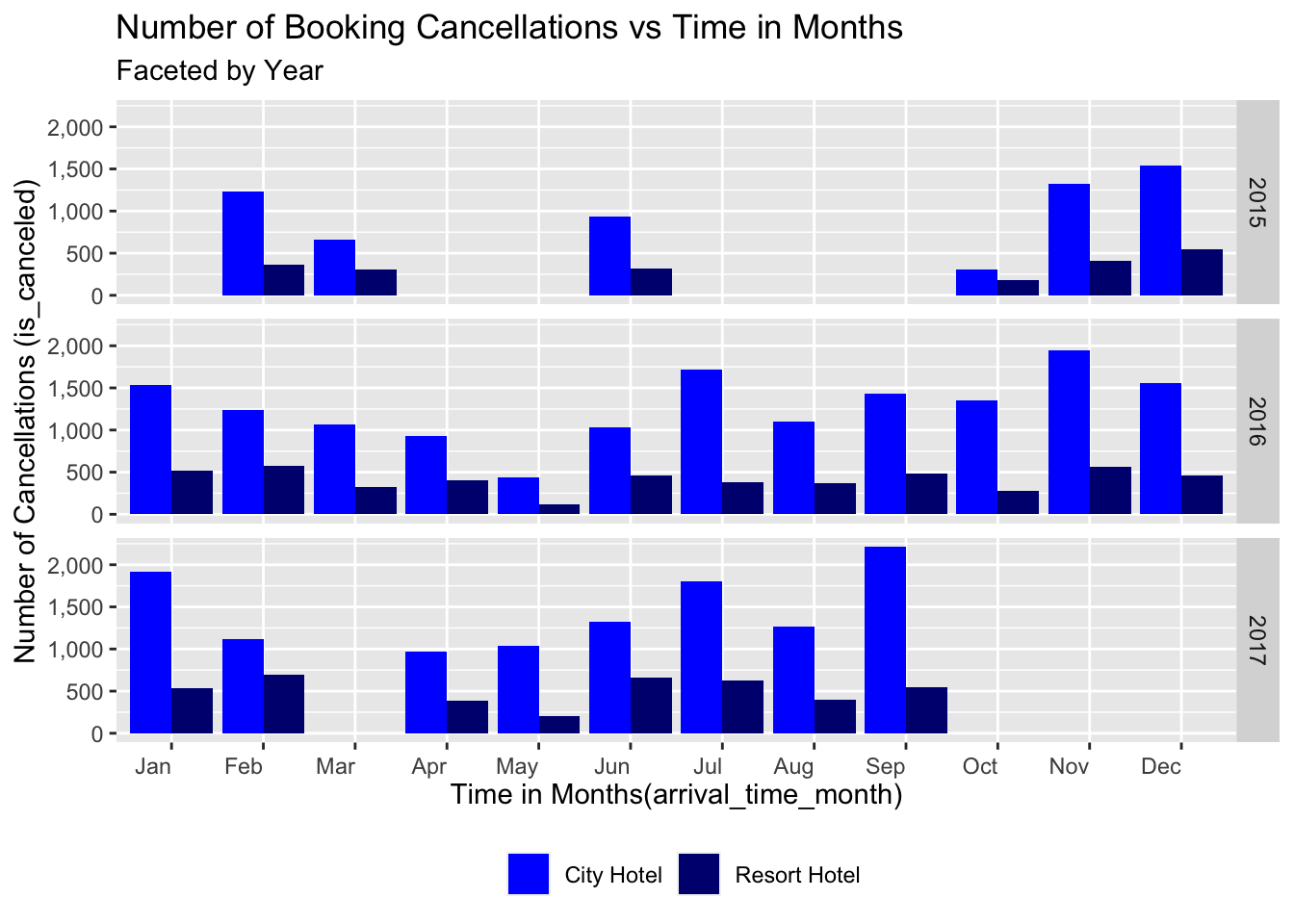
From the given data, we would like to know if there is a higher cancellation rate for the refundable deposit type. Looking at the plot below, we can see that there are three deposit_type: No Deposit, Non-Refundable, and Refundable. As shown in data summary below, the majority type was No Deposit, followed by Non-refundable. A Non-refundable booking is likely to be canceled regardless of hotel types. For bookings with No deposit, the proportion of cancellation in city hotel is slightly higher, but pretty close to that in resort hotel. For Refundable bookings, significantly more cancellations were made in city hotel. Surprisingly, the cancellation rate for the Refundable type is pretty low compared to the other two deposit types. Ideally, the expectation is that since one can get his money back, there would be a higher cancellation rate for the Refundable deposit type as compared to the Non-refundable type where the deposit money is forfeited by the hotel.
data_hotels_factor <- data_hotels
data_hotels_factor$is_canceled <- as.factor(data_hotels_factor$is_canceled)

table(data_hotels_factor$deposit_type)
No Deposit Non Refund Refundable
104238 14587 162 data_hotels_factor%>% ggplot( aes(x=hotel, fill=is_canceled)) +
geom_bar(position="fill") +
scale_fill_manual(values=c("#80CDC1", "#C2A5CF"),labels=c("not canceled", "canceled")) +
guides(fill=guide_legend(title=NULL)) +
facet_grid(. ~ deposit_type) +
theme(legend.position="bottom", axis.text.x=element_text(angle=90, hjust=1, vjust=0.5)) +
labs(x="", y="Cancelation Fraction", title = "Cancelation Fraction vs. Deposit Type ")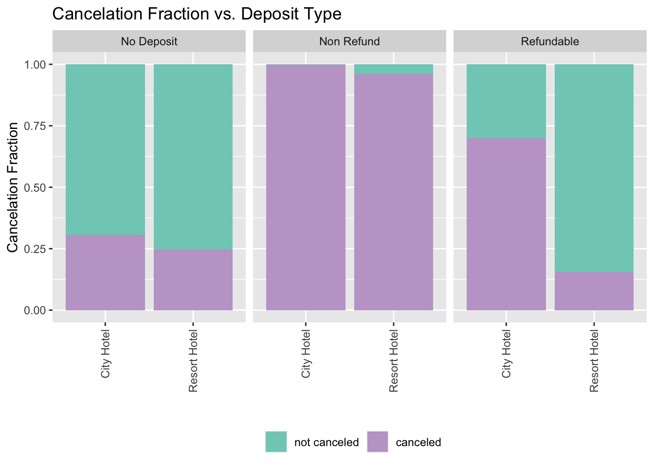
Out of all the market segments, within the ‘Groups’ market the ‘City hotel’ bookings are more likely to be canceled than ‘Resort Hotels’. Similarly, within Offline TA/TO, City hotel bookings are more likely to be canceled than Resort Hotel. However, for Online TA, Corporate and Direct Market, there are no significant difference between the two hotel types(City vs Resort hotels).
data_hotels_factor %>% filter(market_segment %in% c( "complementary", "Corporate", "Direct", "Groups", "Offline TA/TO", "Online TA")) %>%
    ggplot(aes(x=hotel, fill=is_canceled)) +
    geom_bar(position="fill") +
    scale_fill_manual(values=c("#80CDC1", "#C2A5CF"),labels=c("not canceled", "canceled")) + guides(fill=guide_legend(title=NULL)) + facet_grid(. ~ market_segment) + theme(legend.position="bottom", axis.text.x=element_text(angle=90, hjust=1, vjust=0.5))+ labs(x="", y="Cancelation Fraction", title = "Cancelation Fraction vs. Market Segment ")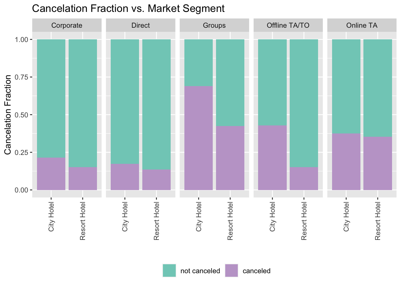
Lastly, the plot below shows the relationship between lead time and the number of cancellations. The lead time for a canceled booking was much longer than that of a booking without cancellation irrespective of the hotel type. Hence hotel reservations made in advance are much more likely to be canceled than reservations made a few days before the the date of arrival.
data_hotels_factor %>%  ggplot(aes(x = hotel, y = lead_time, fill = is_canceled)) +
geom_boxplot(position = position_dodge()) +
scale_fill_manual(values=c("#80CDC1", "#C2A5CF"),labels=c("not canceled", "canceled")) +
labs( title = "Lead time vs. Resort type", x = "Resort Type", y = "Lead Time (days)", subtitle = "Factored by is_canceled")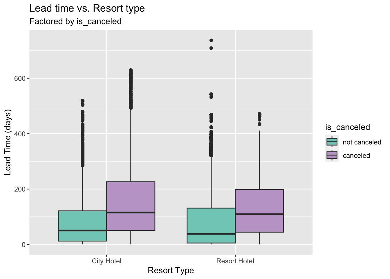
Some of the key insights from the descriptive statistics are:
The mean of the Average Daily Rate($) is 102.01, and the median of the Average Daily Rate is 95 USD.
The reservation status for hotels is; 63% Checked-out, 36% Canceled, and 1% No-show.
BB (Bed & Breakfast) is the most ordered meal which is around 77.3%, followed by HB(Half Board) which is 12.15%, SC(no meal package) which is 8.8%, Undefined and FB (Full Board) which account for the rest.
Roughly half (47.25%) of all the hotel bookings are done via the online TA (Travel Agent). This includes websites like Expedia, and hotels.com. The next major segment is the offline TA (20.32%), which may include bookings done by a human travel agent or in-person bookings. Aviation, Complementary, Corporate, Direct and Groups together contribute to around 1/3 of the total market share.
City hotels have a bimodal distribution for ADR around 60-100 USD. This means that there are some cheaper hotels that are for 60, but there are a few expensive ones that rent for 100 USD. On the other hand, for resort hotels the ADR distribution is much more smooth with a maximum density around 50 USD. From this we can conclude that, on an average, city hotels are more expensive to rent as compared to resort style hotels.
Some of the key insights from the univariate data analysis are:
City Hotels accounts for 66.3% of the total hotel bookings in this dataset whereas resort hotels account for 33.65% of the total hotel bookings.
Hotel bookings are seasonal in nature and peak during the summer months (Jun, Jul, Aug) and the winter holiday season (Nov, Dec, Jan).
The highest number of bookings are done from the top 3 countries of Portugal(PRT), Great Britain(GBR) and France (FRA) respectively.
The median length of stay per booking is 3 days. The mean is 3.45 days.
The median number of guests per booking is 2.
It is cheaper to rent a hotel room if it is booked in advance(~ 20-30 days) but this trend is more prevalent for resort hotels than city hotels.
There is an increase in the Average Daily Rate (ADR) during the start(1st) and end of the month (30th-31st). Hence if we want to rent a room for a cheaper price, it is best to avoid the start and end of the month as the arrival date.
Transient customer (i.e. individual guests not belonging to any group or corporation ) are much more likely (3x) to cancel their hotel reservations as compared to other customer types.
Cancellations are seasonal as well and peak during the summer months (Jun, Jul, Aug) and the winter holiday season (Nov, Dec, Jan). For the summer season there is an increased likelihood of people their flights/trains during busy summer season. On the other hand, during the Christmas season there is the added chance of inclement snowy weather that can increase the cancellation rate.
Surprisingly, the cancellation rate for the Refundable deposit type is pretty low (~40%) compared to the Non-refundable(~96%). Ideally, the expectation is that since one can get his money back, there would be a higher cancellation rate for the Refundable deposit type as compared to the Non-refundable type where the deposit money is forfeited by the hotel.
City hotel bookings are more likely to be canceled than ‘Resort Hotels’ in the ‘Groups’ and ‘Offline TA/TO’ market segment. However, for Online TA, Corporate and Direct Market, there are no significant difference between the two hotel types(City vs Resort hotels).
Hotel reservations made in advance are much more likely to be canceled than reservations made a few days before the the date of arrival for both hotel types.
In summary, the hotel_bookings.csv provides a lot of key insights into the hotel industry. From the dataset provided to us, we have graphically proven that it is cheaper to rent a hotel room if it is booked in advance(~ 20-30 days). Also, there is an increase in the Average Daily Rate (ADR) during the start(1st) and end of the month (30th-31st). Hence if we want to rent a room for a cheaper price, it is best to avoid the start and end of the month as the arrival date.
We also learned about a surprising trend that the cancellation rate for the Refundable deposit type is pretty low (~40%) compared to the Non-refundable(~96%) deposit booking which is contrary to expectation since one can get his money back for Refundable deposits. Ideally, there should be a higher cancellation rate for the Refundable deposit type as compared to the Non-refundable type since for Non-refundable deposits, the deposit money is forfeited by the hotel. Lastly, we were also able to prove visually that hotel reservations made in advance are much more likely to be canceled than reservations made a few days before the the date of arrival for both hotel types. Learning from these trends, the hotel industry can alter their business practices by providing adequate incentives and benefits in order to prevent cancellations. They can also be better prepared to tackle the seasonal demand of the hotel bookings. Using the hotel_bookings dataset, we have successfully identified the hidden trends in the booking data. In conclusion, data-driven decision-making allows for a better understanding of business needs by leveraging real, verified data, instead of just making assumptions. This in turn boosts profitability and promotes organizations to make well-informed decision instead of take a shot in the dark.
Overall, the hotel_bookings.csv dataset is a comprehensive dataset which a lot of columns. This helps us in finding key insights for different variables for different hotel bookings. But there are some limitations for the dataset. They are capitulated in the bullet points below:
Although there are enough variables in the data set, I think we could have derived an in depth understanding of the data using a few more variables like ‘purpose_of_visit’, ‘age’, ‘gender’, ‘city’,‘proximity_to_public_transport’ etc.
Some of the observations in the dataset are erroneous and contain zero adults but they have non-zero children and babies. This is obviously wrong since children and babies are not allowed to book/check-in to a hotel on their own. Removing these observations leads to missing data in our dataset.
The hotel_bookings.csv dataset only contains data for three years (2015-2017). While that is enough to get a preliminary idea of the trends in the hotel industry, in order to make stronger and more accurate predictions, we need to have access to data that is longer than 3 years (around 10-15 years). This is because the hotel industry goes through macroeconomic cycles which have a span of 3-5 years. For e.g. if we consider the hotel data for just three years during the COVID pandemic from 2019-2021, then the booking rate will be on the lower side since there were major travel bans across cities and countries and hence the total number of bookings during COVID would be much lower. But now if we were to make future assumption (for 2023) using that data, then we get erroneous predictions since the hotel industry had a significant recovery post-pandemic.
To improve on this project in the future, I would work on some of the shortcomings addressed above in the Limitation section.
Although this project provides a good preliminary glance at the hotel industry, we can an in-depth understanding of the data using a few more variables like ‘purpose_of_visit’, ‘age’, ‘gender’, ‘city’,‘proximity_to_public_transport’ etc.
Finding a dataset that has lower number of erroneous observations.
Obtaining longer time trends for the data set. The current dataset is for three years (2015-2017), but in order to make more accurate predictions we need to have access to data that is longer than 3 years (around 10-15 years).
The source of the dataset for this final report is: https://www.kaggle.com/datasets/jessemostipak/hotel-booking-demand.
https://www.sciencedirect.com/science/article/pii/S2352340918315191
Wickham, H., & Grolemund, G. (2016). R for data science: Visualize, model, transform, tidy, and import data. https://r4ds.had.co.nz
R Core Team (2023). R: A Language and Environment for Statistical Computing. R Foundation for Statistical Computing, Vienna, Austria. https://www.R-project.org/.