library(tidyverse)
library(ggplot2)
library(readxl)
knitr::opts_chunk$set(echo = TRUE, warning=FALSE, message=FALSE)
Challenge 7 Submission
challenge_7
air_bnb
Visualizing Multiple Dimensions
Challenge Overview
Today’s challenge is to:
- read in a data set, and describe the data set using both words and any supporting information (e.g., tables, etc)
- tidy data (as needed, including sanity checks)
- mutate variables as needed (including sanity checks)
- Recreate at least two graphs from previous exercises, but introduce at least one additional dimension that you omitted before using ggplot functionality (color, shape, line, facet, etc) The goal is not to create unneeded chart ink (Tufte), but to concisely capture variation in additional dimensions that were collapsed in your earlier 2 or 3 dimensional graphs.
- Explain why you choose the specific graph type
- If you haven’t tried in previous weeks, work this week to make your graphs “publication” ready with titles, captions, and pretty axis labels and other viewer-friendly features
R Graph Gallery is a good starting point for thinking about what information is conveyed in standard graph types, and includes example R code. And anyone not familiar with Edward Tufte should check out his fantastic books and courses on data visualizaton.
(be sure to only include the category tags for the data you use!)
Read in data
Read in one (or more) of the following datasets, using the correct R package and command.
- air_bnb ⭐⭐⭐
Ans: I had used the debt_in_trillions.xlsx data set in the last challenge(#6), but unfortunately challenge 7 doesn’t have that data set. So instead I will be using the AB_NYC_2019.csv dataset which contains all the airbnb listings.
airbnb <- read_csv("_data/AB_NYC_2019.csv")
airbnb
Briefly describe the data
Ans: Looking at the glimpse function below, we can see that the airbnb data set has 48,895 rows x 16 cols. It shows the airbnb listing information for the city of New York for the year 2019. We can also see the column names and data types for each column below.
glimpse(airbnb)Rows: 48,895
Columns: 16
$ id <dbl> 2539, 2595, 3647, 3831, 5022, 5099, 512…
$ name <chr> "Clean & quiet apt home by the park", "…
$ host_id <dbl> 2787, 2845, 4632, 4869, 7192, 7322, 735…
$ host_name <chr> "John", "Jennifer", "Elisabeth", "LisaR…
$ neighbourhood_group <chr> "Brooklyn", "Manhattan", "Manhattan", "…
$ neighbourhood <chr> "Kensington", "Midtown", "Harlem", "Cli…
$ latitude <dbl> 40.64749, 40.75362, 40.80902, 40.68514,…
$ longitude <dbl> -73.97237, -73.98377, -73.94190, -73.95…
$ room_type <chr> "Private room", "Entire home/apt", "Pri…
$ price <dbl> 149, 225, 150, 89, 80, 200, 60, 79, 79,…
$ minimum_nights <dbl> 1, 1, 3, 1, 10, 3, 45, 2, 2, 1, 5, 2, 4…
$ number_of_reviews <dbl> 9, 45, 0, 270, 9, 74, 49, 430, 118, 160…
$ last_review <date> 2018-10-19, 2019-05-21, NA, 2019-07-05…
$ reviews_per_month <dbl> 0.21, 0.38, NA, 4.64, 0.10, 0.59, 0.40,…
$ calculated_host_listings_count <dbl> 6, 2, 1, 1, 1, 1, 1, 1, 1, 4, 1, 1, 3, …
$ availability_365 <dbl> 365, 355, 365, 194, 0, 129, 0, 220, 0, …We are primarily interested in the room_type and neighborhood_group columns. Looking at the code below, we can see that there are three room types with entire home/apt and private rooms being the dominant category. Also we can see that there are five boroughs/neighbourhoods in New York with Brooklyn and Manhattan having the most number of airbnb properties.
print("Airbnb room type")[1] "Airbnb room type"table(airbnb$room_type)
Entire home/apt    Private room     Shared room
25409 22326 1160 print("Airbnb neighbourhoods")[1] "Airbnb neighbourhoods"table(airbnb$neighbourhood_group)
        Bronx      Brooklyn     Manhattan        Queens Staten Island
         1091         20104         21661          5666           373
Tidy Data (as needed)
Is your data already tidy, or is there work to be done? Be sure to anticipate your end result to provide a sanity check, and document your work here.
Ans: Each airbnb listing has its own row in the airbnb data set above and hence the data is already in a tidy format.
Are there any variables that require mutation to be usable in your analysis stream? For example, do you need to calculate new values in order to graph them? Can string values be represented numerically? Do you need to turn any variables into factors and reorder for ease of graphics and visualization?
Document your work here.
Ans: Yes, we need to convert some of the columns into factor so that its easier for data visualization. Also we are only concerned with the year part of the date for the data visualization. Hence we need to create a new column containing only the year. The code for that is given below:
airbnb_factored <- airbnb %>%
  mutate(room_type = as_factor(room_type),
         neighbourhood_group = as_factor(neighbourhood_group),
         neighbourhood = as_factor(neighbourhood))

airbnb_factored <- airbnb_factored %>% mutate(year = year(last_review))
Visualization with Multiple Dimensions
Ans: I didn’t use the airbnb data set for challenge 6 but the two graphs I plotted were a time trend (total debt vs year) and a stacked area chart showing each debt type vs year. Here, we can continue the same data visualization techniques and plot a time trend of the airbnb properties vs year split by neighbourhood_group which would be the third dimension.
airbnb_grouped <- airbnb_factored %>%
  group_by(year,neighbourhood_group) %>%
  summarize(num_prop = n_distinct(id)) %>%
  filter(!is.na(year))

ggplot(airbnb_grouped,aes(x=year,y=num_prop,col=neighbourhood_group)) + geom_line() + labs(x="Year of Last Review",y="Number of Airbnb Properties",title="Number of Airbnb Properties v/s Year") + scale_x_continuous(breaks = c(2011,2012,2013,2014,2015,2016,2017,2018,2019), labels = c("2011","2012","2013","2014","2015","2016","2017","2018","2019")) + theme(axis.text.x=element_text(angle=60, hjust=1))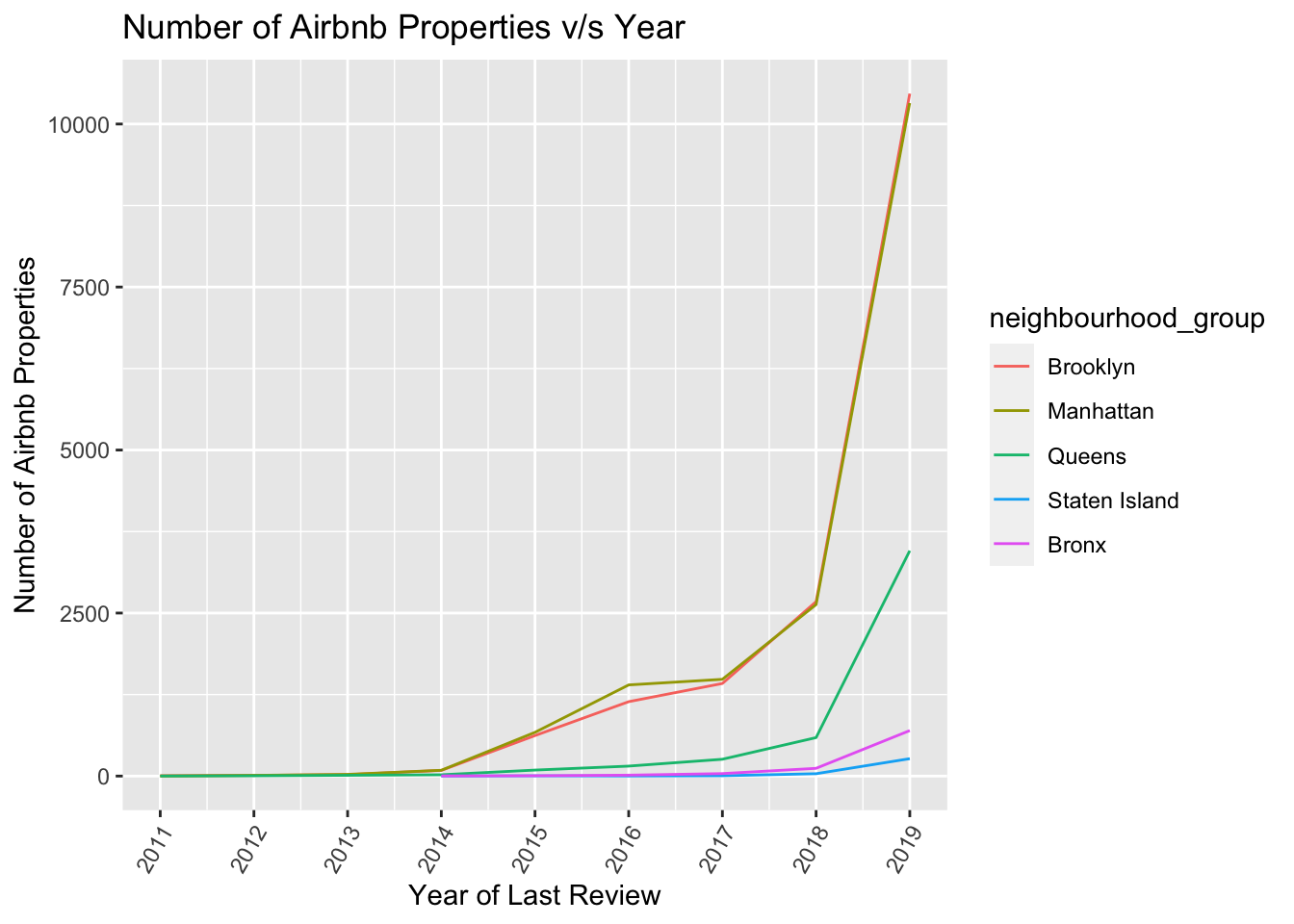
From the above plot we can see that there has been a sharp spike in the number for listing for Brooklyn and Manhattan from 2017-2019. We can use facet_wrap to split each group.
ggplot(airbnb_grouped,aes(x=year,y=num_prop)) + geom_line() + labs(x="Year of Last Review",y="Number of airbnb properties",title="Airbnb Properties v/s Year",subtitle="Number of Airbnb Properties vs the Year of Last Review") + scale_x_continuous(breaks = c(2011,2012,2013,2014,2015,2016,2017,2018,2019), labels = c("2011","2012","2013","2014","2015","2016","2017","2018","2019")) + theme(axis.text.x=element_text(angle=60, hjust=1)) + facet_wrap(~neighbourhood_group)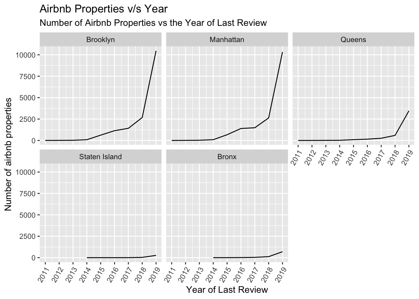
In challenge 6, I plotted a stacked area chart. Here we can plot a stacked bar chart by comparing the average daily price($) on the y-axis to neighborhood on the x-axis and split it by the room_type(3rd dimension). From the plot below we can conclude that on an average, Manhattan is most expensive neighborhood for all room types. Also, we see a general trend across all the boroughs that entire home/apts are the most expensive to rent followed by private room and shared room.
airbnb_grouped2<- airbnb_factored %>% group_by(room_type,neighbourhood_group) %>% summarize(avg_price=mean(price))

ggplot(airbnb_grouped2,aes(x=neighbourhood_group,y=avg_price,fill=room_type)) + geom_col(position="dodge") + labs(x="neighbourhood_group",y="Average Daily Rental Price($)",title="Average Daily Rental Price($) v/s Neighbourhood Group") + theme(axis.text.x=element_text(angle=90, hjust=1)) 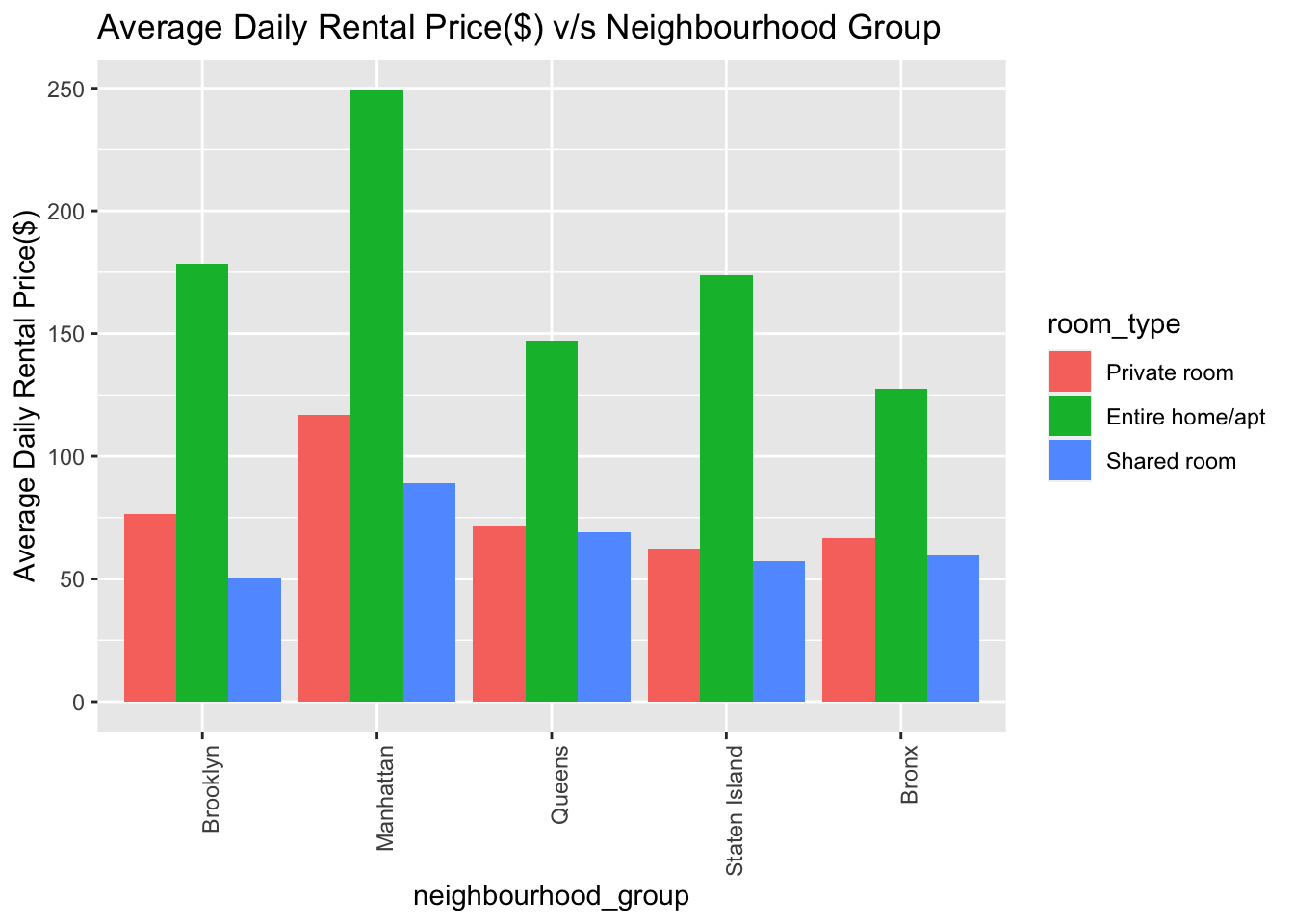
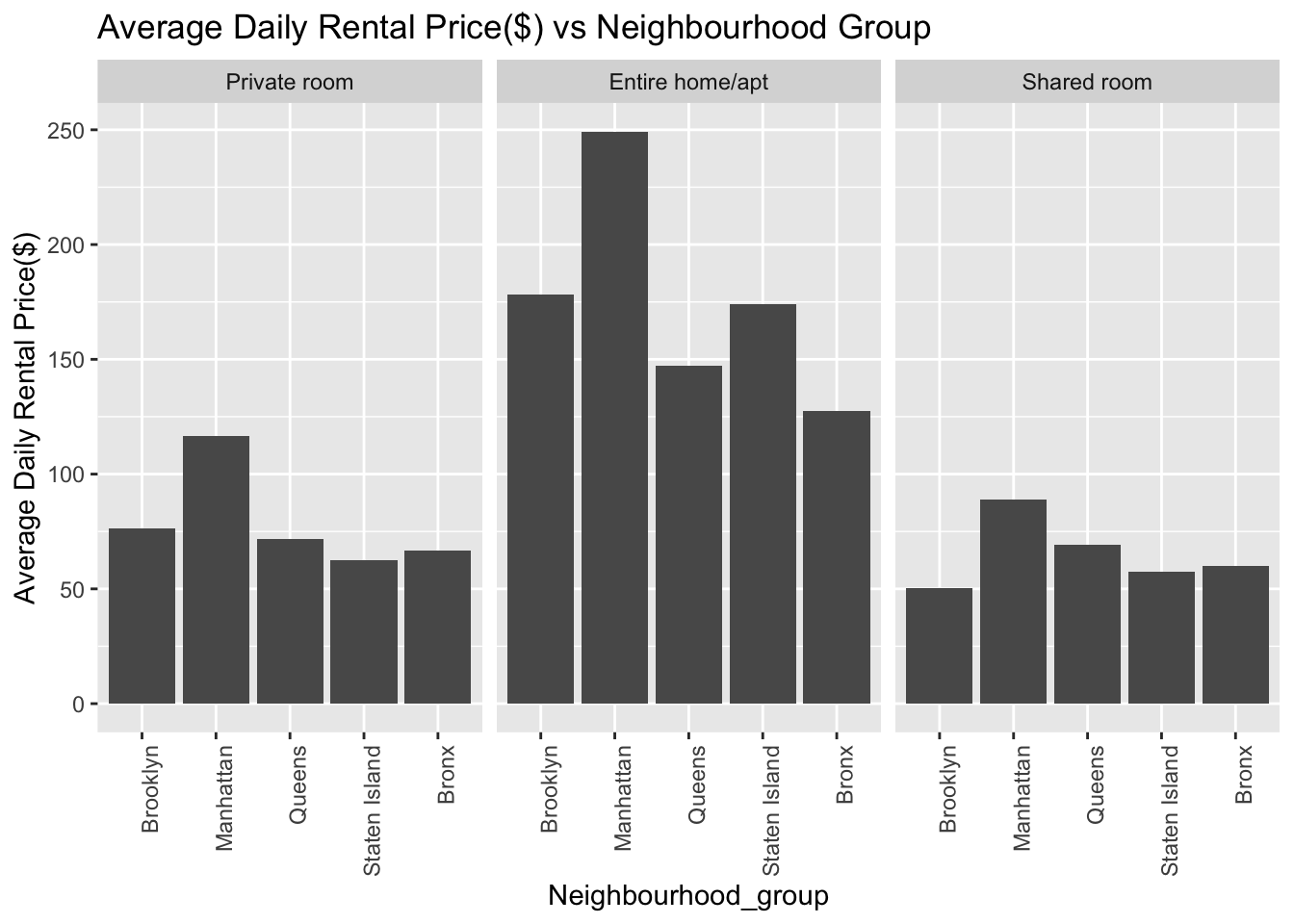
We can also split the above bar chart by room_type using the facet_wrap function. The code for that is given below. We see the same trend here. Manhattan is most expensive neighborhood for all room types. Also, we see a general trend across all the boroughs that entire home/apts are the most expensive to rent followed by private room and then shared room.
ggplot(airbnb_grouped2,aes(x=neighbourhood_group,y=avg_price)) + geom_col(position="dodge") + labs(x="Neighbourhood_group",y="Average Daily Rental Price($)",title="Average Daily Rental Price($) vs Neighbourhood Group") + theme(axis.text.x=element_text(angle=90, hjust=1)) +facet_wrap(~room_type)