library(tidyverse)
library(ggplot2)

knitr::opts_chunk$set(echo = TRUE, warning=FALSE, message=FALSE)
Challenge 8 Submission
challenge_8
snl
Joining Data
Challenge Overview
Today’s challenge is to:
- read in multiple data sets, and describe the data set using both words and any supporting information (e.g., tables, etc)
- tidy data (as needed, including sanity checks)
- mutate variables as needed (including sanity checks)
- join two or more data sets and analyze some aspect of the joined data
(be sure to only include the category tags for the data you use!)
Read in data
Read in one (or more) of the following datasets, using the correct R package and command.
- snl ⭐⭐⭐⭐⭐
Ans: For challenge 8, I am going to use the three snl datasets. The code to read the datasets is given below:
snl_actors <- read_csv("_data/snl_actors.csv")
snl_actors
snl_casts <- read_csv("_data/snl_casts.csv")
snl_castssnl_seasons <- read_csv("_data/snl_seasons.csv")
snl_seasonsBriefly describe the data
Ans The snl_actors dataset contains 2,306 rows x 4 cols. The description and datatype for each column is given in the code cell below:
glimpse(snl_actors)Rows: 2,306
Columns: 4
$ aid <chr> "Kate McKinnon", "Alex Moffat", "Ego Nwodim", "Chris Redd", "Ke…
$ url <chr> "/Cast/?KaMc", "/Cast/?AlMo", "/Cast/?EgNw", "/Cast/?ChRe", "/C…
$ type <chr> "cast", "cast", "cast", "cast", "cast", "guest", "guest", "cast…
$ gender <chr> "female", "male", "unknown", "male", "male", "andy", "male", "f…The snl_casts dataset contains 614 rows x 8 cols. The description and datatype for each column is given in the code cell below. Notice that both the snl_actors and snl_casts have the aid column common to both the data sets. We will be using this to join the datasets.
glimpse(snl_casts)Rows: 614
Columns: 8
$ aid <chr> "A. Whitney Brown", "A. Whitney Brown", "A. Whitney Br…
$ sid <dbl> 11, 12, 13, 14, 15, 16, 5, 39, 40, 41, 42, 45, 46, 21,…
$ featured <lgl> TRUE, TRUE, TRUE, TRUE, TRUE, TRUE, TRUE, TRUE, TRUE, …
$ first_epid <dbl> 19860222, NA, NA, NA, NA, NA, 19800409, 20140118, NA, …
$ last_epid <dbl> NA, NA, NA, NA, NA, NA, NA, NA, NA, NA, NA, NA, NA, NA…
$ update_anchor <lgl> FALSE, FALSE, FALSE, FALSE, FALSE, FALSE, FALSE, FALSE…
$ n_episodes <dbl> 8, 20, 13, 20, 20, 20, 5, 11, 21, 21, 21, 18, 17, 20, …
$ season_fraction <dbl> 0.4444444, 1.0000000, 1.0000000, 1.0000000, 1.0000000,…The snl_seasons dataset contains 46 rows x 5 cols. The description and datatype for each column is given in the code cell below. Notice that both the snl_casts and snl_seasons have the sid column common to both the data sets. We will be using this to join the datasets.
glimpse(snl_seasons)Rows: 46
Columns: 5
$ sid <dbl> 1, 2, 3, 4, 5, 6, 7, 8, 9, 10, 11, 12, 13, 14, 15, 16, 17, …
$ year <dbl> 1975, 1976, 1977, 1978, 1979, 1980, 1981, 1982, 1983, 1984,…
$ first_epid <dbl> 19751011, 19760918, 19770924, 19781007, 19791013, 19801115,…
$ last_epid <dbl> 19760731, 19770521, 19780520, 19790526, 19800524, 19810411,…
$ n_episodes <dbl> 24, 22, 20, 20, 20, 13, 20, 20, 19, 17, 18, 20, 13, 20, 20,…Tidy Data (as needed)
Is your data already tidy, or is there work to be done? Be sure to anticipate your end result to provide a sanity check, and document your work here.
Ans: Each variable has its own column and each observation has its own row for all three datasets. Hence the data is already in tidy format.
Are there any variables that require mutation to be usable in your analysis stream? For example, do you need to calculate new values in order to graph them? Can string values be represented numerically? Do you need to turn any variables into factors and reorder for ease of graphics and visualization?
Document your work here.
Ans: Yes, we need to change/rename three column names in snl_casts and snl_seasons in this case since they have the same name. If kept unaltered, the final column names in the joined dataset will be ‘first_epid.x’ and ‘first_epid.y’. Hence in order to prevent this issue, we need to rename it. The code for renaming the columns is given below:
snl_casts <- rename(snl_casts,first_epid_casts = first_epid,last_epid_casts=last_epid,n_episodes_casts=n_episodes)

snl_seasons <- rename(snl_seasons,first_epid_seasons = first_epid,last_epid_seasons=last_epid,n_episodes_seasons=n_episodes)
Join Data
Be sure to include a sanity check, and double-check that case count is correct!
Ans: To join the the three datasets, we will be using the ‘aid’ column from ‘snl_actors’ and ‘snl_casts’. For the ‘snl_casts’ and ‘snl_seasons’ dataset, we will be using the ‘sid’ column. In this new merged (joined) dataset we want to only record observations which are common to all three datasets (‘snl_actors’,snl_casts,snl_seasons) and hence we will be using the ‘inner_join’ method.
snl_joined <- snl_casts %>%
  inner_join(snl_actors,by="aid") %>%
  inner_join(snl_seasons,by="sid")

snl_joinedglimpse(snl_joined)Rows: 614
Columns: 15
$ aid <chr> "A. Whitney Brown", "A. Whitney Brown", "A. Whitney…
$ sid <dbl> 11, 12, 13, 14, 15, 16, 5, 39, 40, 41, 42, 45, 46, …
$ featured <lgl> TRUE, TRUE, TRUE, TRUE, TRUE, TRUE, TRUE, TRUE, TRU…
$ first_epid_casts <dbl> 19860222, NA, NA, NA, NA, NA, 19800409, 20140118, N…
$ last_epid_casts <dbl> NA, NA, NA, NA, NA, NA, NA, NA, NA, NA, NA, NA, NA,…
$ update_anchor <lgl> FALSE, FALSE, FALSE, FALSE, FALSE, FALSE, FALSE, FA…
$ n_episodes_casts <dbl> 8, 20, 13, 20, 20, 20, 5, 11, 21, 21, 21, 18, 17, 2…
$ season_fraction <dbl> 0.4444444, 1.0000000, 1.0000000, 1.0000000, 1.00000…
$ url <chr> "/Cast/?AWBr", "/Cast/?AWBr", "/Cast/?AWBr", "/Cast…
$ type <chr> "cast", "cast", "cast", "cast", "cast", "cast", "ca…
$ gender <chr> "male", "male", "male", "male", "male", "male", "ma…
$ year <dbl> 1985, 1986, 1987, 1988, 1989, 1990, 1979, 2013, 201…
$ first_epid_seasons <dbl> 19851109, 19861011, 19871017, 19881008, 19890930, 1…
$ last_epid_seasons <dbl> 19860524, 19870523, 19880227, 19890520, 19900519, 1…
$ n_episodes_seasons <dbl> 18, 20, 13, 20, 20, 20, 20, 21, 21, 21, 21, 18, 17,…Looking at the glimpse function, we can see that the joined dataset has the size 614 rows x 15 cols.
Data Analysis
Ans: From the joined dataset we can plot the gender characteristics of the snl cast for every year. First, we need to process the snl_joined dataset and group it by year and gender to get the relevant characteristics. We then mutate the dataset to add a percentage column. The code is given below:
gender_groupby <- snl_joined %>%
group_by(year,gender) %>%
summarize(num_gender = n_distinct(aid)) %>%
ungroup() %>%
group_by(year) %>%
mutate(percentage = 100*(num_gender/sum(num_gender)))
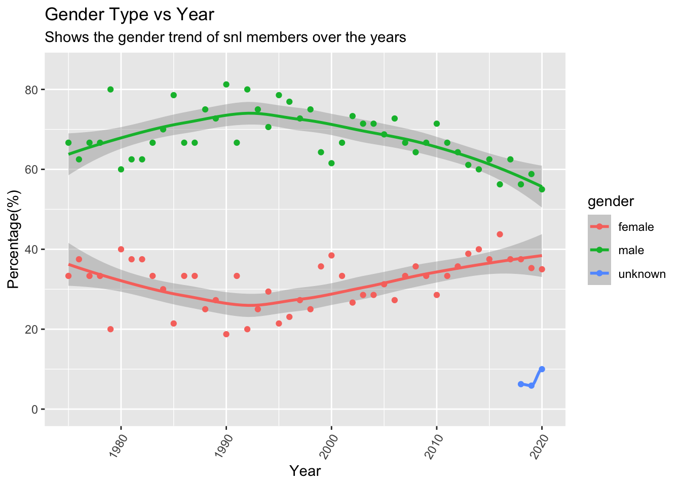
gender_groupbyNow we can now plot a graph of the gender diversity vs time (in years). Looking at the plot below, we can conclude that at the start (1975) there were around 65% male members which gradually kept on increasing till it reached a peak around 1992-1993. From there, the percentage of males has been dropping and the share of female snl members has been increasing up until 2020. We also see that there is a third gender category for the recent years of 2017-2020. This could include people who do not conform to the binary gender category (e.g. trans, non-binary etc.).
ggplot(gender_groupby,aes(x=year,y=percentage,color=gender)) + geom_smooth() + geom_point() + labs(x="Year",y="Percentage(%)",title="Gender Type vs Year",subtitle ="Shows the gender trend of snl members over the years") + ylim(0,85)+ theme(axis.text.x=element_text(angle=60, hjust=1))