Challenge 10 Post: Using Purr with the Aninal Weight Data

challenge_10

purrr

Author

Hunter Major

Published

July 9, 2023

Challenge Overview

The purrr package is a powerful tool for functional programming. It allows the user to apply a single function across multiple objects. It can replace for loops with a more readable (and often faster) simple function call.

For example, we can draw n random samples from 10 different distributions using a vector of 10 means.

n <- 100 # sample size
m <- seq(1,10) # means 
samps <- map(m,rnorm,n=n)

We can then use map_dbl to verify that this worked correctly by computing the mean for each sample.

samps %>%
  map_dbl(mean)

 [1] 1.165970 2.131546 3.081201 4.069321 4.910645 6.153407 6.957024 8.056468
 [9] 8.952136 9.954956

purrr is tricky to learn (but beyond useful once you get a handle on it). Therefore, it’s imperative that you complete the purr and map readings before attempting this challenge.

The challenge

Use purrr with a function to perform some data science task. What this task is is up to you. It could involve computing summary statistics, reading in multiple datasets, running a random process multiple times, or anything else you might need to do in your work as a data analyst. You might consider using purrr with a function you wrote for challenge 9.

Reading in the Data

For this challenge, I am going to read in the animal_weight.csv dataset.

animalweight1 <- read.csv("_data/animal_weight.csv")
animalweight1

Solution

We can split the animal weight dataset based on IPCC.Area, which would return 9 datasets for each of the 9 IPCC.Areas, which are large(r) global regions.

animalweight2_area <- split(animalweight1, animalweight1$IPCC.Area)
animalweight2_area

$Africa
  IPCC.Area Cattle...dairy Cattle...non.dairy Buffaloes Swine...market
3    Africa            275                173       380             28
  Swine...breeding Chicken...Broilers Chicken...Layers Ducks Turkeys Sheep
3               28                0.9              1.8   2.7     6.8    28
  Goats Horses Asses Mules Camels Llamas
3    30    238   130   130    217    217

$Asia
  IPCC.Area Cattle...dairy Cattle...non.dairy Buffaloes Swine...market
7      Asia            350                391       380             50
  Swine...breeding Chicken...Broilers Chicken...Layers Ducks Turkeys Sheep
7              180                0.9              1.8   2.7     6.8  48.5
  Goats Horses Asses Mules Camels Llamas
7  38.5    377   130   130    217    217

$`Eastern Europe`
       IPCC.Area Cattle...dairy Cattle...non.dairy Buffaloes Swine...market
2 Eastern Europe            550                391       380             50
  Swine...breeding Chicken...Broilers Chicken...Layers Ducks Turkeys Sheep
2              180                0.9              1.8   2.7     6.8  48.5
  Goats Horses Asses Mules Camels Llamas
2  38.5    377   130   130    217    217

$`Indian Subcontinent`
            IPCC.Area Cattle...dairy Cattle...non.dairy Buffaloes
1 Indian Subcontinent            275                110       295
  Swine...market Swine...breeding Chicken...Broilers Chicken...Layers Ducks
1             28               28                0.9              1.8   2.7
  Turkeys Sheep Goats Horses Asses Mules Camels Llamas
1     6.8    28    30    238   130   130    217    217

$`Latin America`
      IPCC.Area Cattle...dairy Cattle...non.dairy Buffaloes Swine...market
6 Latin America            400                305       380             28
  Swine...breeding Chicken...Broilers Chicken...Layers Ducks Turkeys Sheep
6               28                0.9              1.8   2.7     6.8    28
  Goats Horses Asses Mules Camels Llamas
6    30    238   130   130    217    217

$`Middle east`
    IPCC.Area Cattle...dairy Cattle...non.dairy Buffaloes Swine...market
8 Middle east            275                173       380             28
  Swine...breeding Chicken...Broilers Chicken...Layers Ducks Turkeys Sheep
8               28                0.9              1.8   2.7     6.8    28
  Goats Horses Asses Mules Camels Llamas
8    30    238   130   130    217    217

$`Northern America`
         IPCC.Area Cattle...dairy Cattle...non.dairy Buffaloes Swine...market
9 Northern America            604                389       380             46
  Swine...breeding Chicken...Broilers Chicken...Layers Ducks Turkeys Sheep
9              198                0.9              1.8   2.7     6.8  48.5
  Goats Horses Asses Mules Camels Llamas
9  38.5    377   130   130    217    217

$Oceania
  IPCC.Area Cattle...dairy Cattle...non.dairy Buffaloes Swine...market
4   Oceania            500                330       380             45
  Swine...breeding Chicken...Broilers Chicken...Layers Ducks Turkeys Sheep
4              180                0.9              1.8   2.7     6.8  48.5
  Goats Horses Asses Mules Camels Llamas
4  38.5    377   130   130    217    217

$`Western Europe`
       IPCC.Area Cattle...dairy Cattle...non.dairy Buffaloes Swine...market
5 Western Europe            600                420       380             50
  Swine...breeding Chicken...Broilers Chicken...Layers Ducks Turkeys Sheep
5              198                0.9              1.8   2.7     6.8  48.5
  Goats Horses Asses Mules Camels Llamas
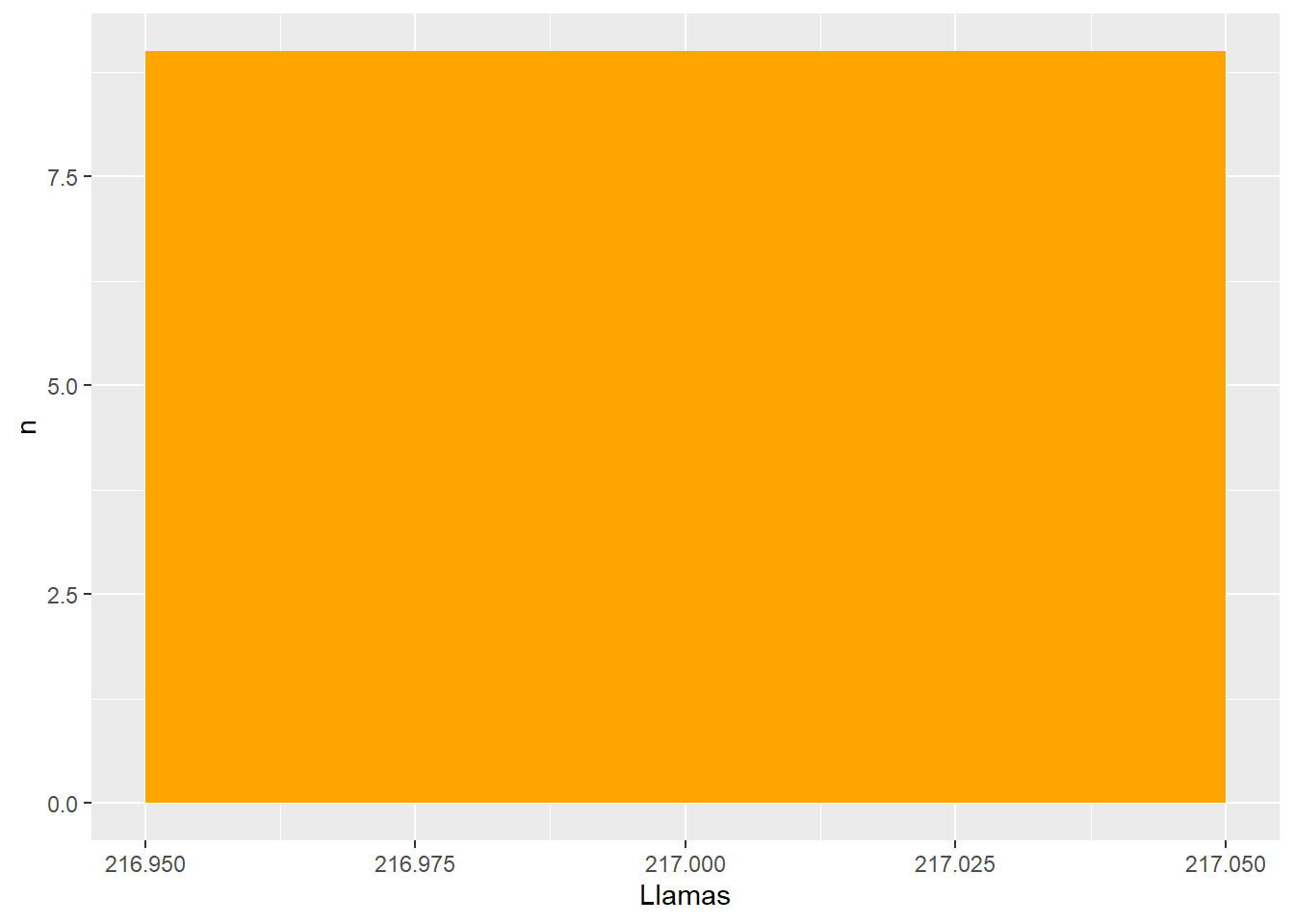
5  38.5    377   130   130    217    217

In Challenge 9, I created a function that could build a histogram for a variable which I will rework with slight adjustments below, this time using purr’s map () to help visualize the histograms for Cattle (dairy and non-dairy), Swine (market and breeding), Buffaloes, Sheep, Turkeys, Ducks, Horses, Goats, and Llamas. ## Function for Histogram

# Creating a function, build_histogram, to make a histogram
build_histogram <- function(data, col_name, title, fill="orange", xlab="x", ylab= "n") {
  col_name <- rlang::ensym(col_name)
  data %>%
    ggplot(aes({{col_name}})) + geom_histogram(fill= fill)+ labs(x=col_name, y=ylab)
}

Building Histogram

# building the histogram using map()
map(c("Cattle...dairy", "Cattle...non.dairy", "Buffaloes", "Swine...market", "Swine...breeding", "Sheep", "Turkeys", "Ducks", "Goats", "Horses", "Llamas"), ~build_histogram(dat=animalweight1, col_name=!!.x))

[[1]]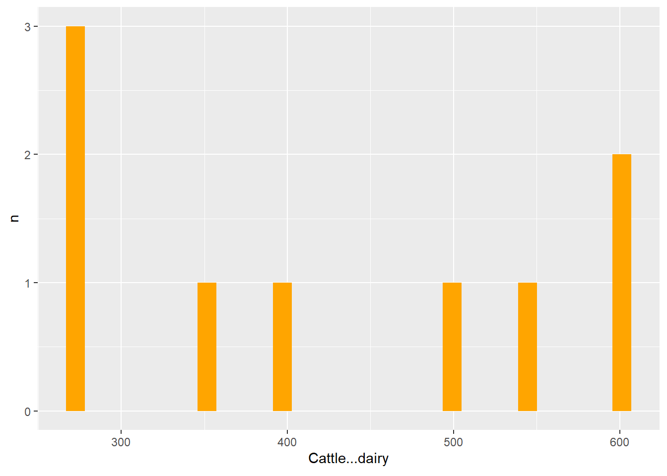


[[2]]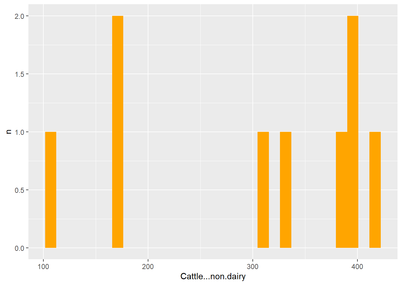


[[3]]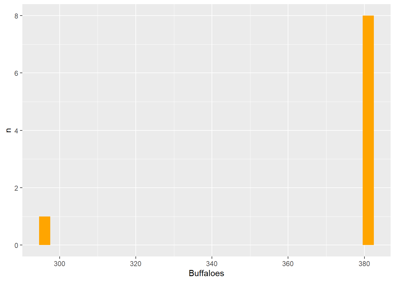


[[4]]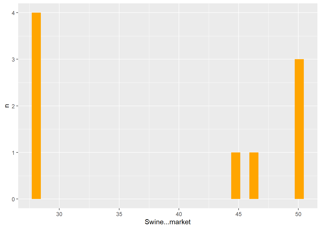


[[5]]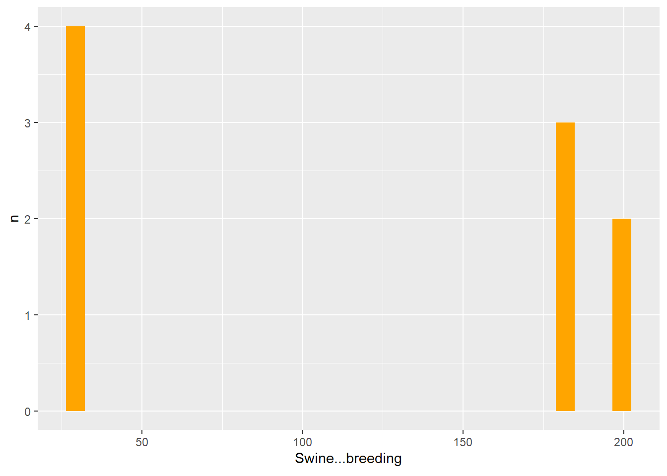


[[6]]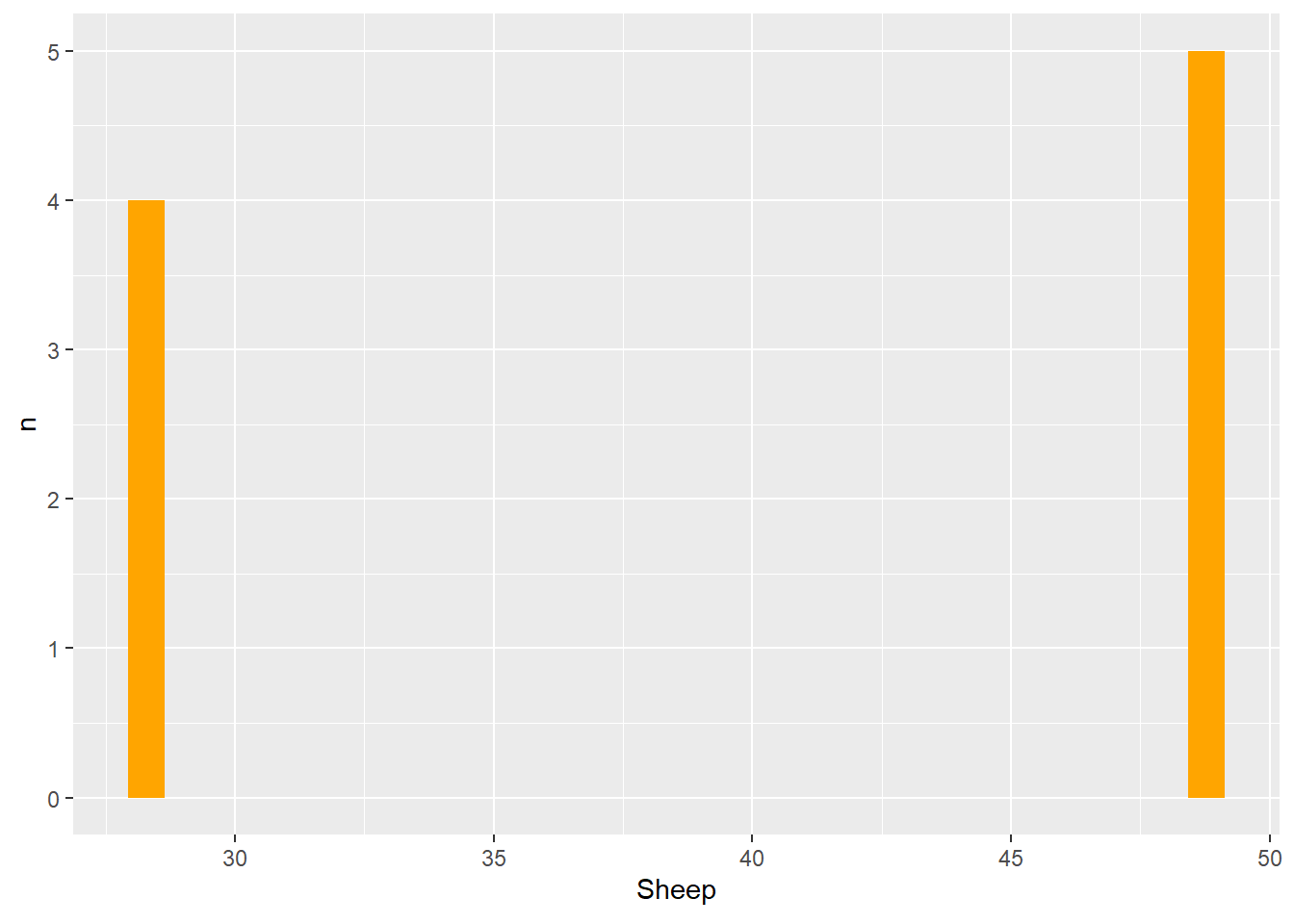


[[7]]


[[8]]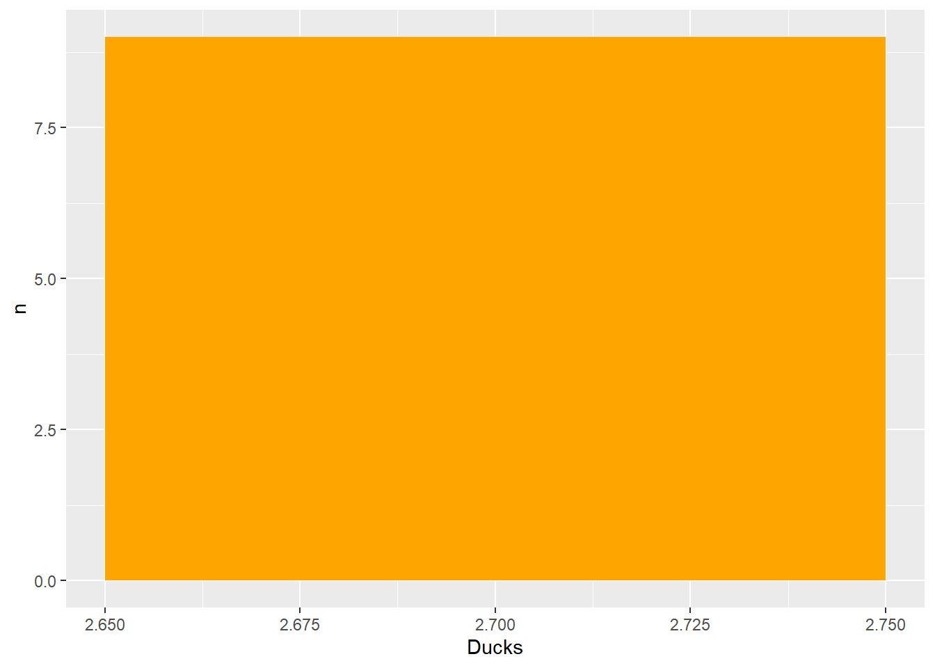


[[9]]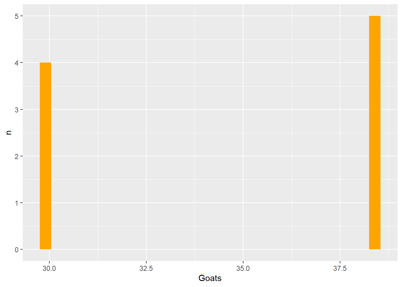


[[10]]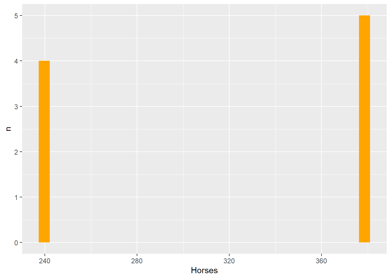


[[11]]