The purrr package is a powerful tool for functional programming. It allows the user to apply a single function across multiple objects. It can replace for loops with a more readable (and often faster) simple function call.
For example, we can draw n random samples from 10 different distributions using a vector of 10 means.
n <-100# sample sizem <-seq(1,10) # means samps <-map(m,rnorm,n=n) samps
purrr is tricky to learn (but beyond useful once you get a handle on it). Therefore, it’s imperative that you complete the purr and map readings before attempting this challenge.
The challenge
Use purrr with a function to perform some data science task. What this task is is up to you. It could involve computing summary statistics, reading in multiple datasets, running a random process multiple times, or anything else you might need to do in your work as a data analyst. You might consider using purrr with a function you wrote for challenge 9.
Solutions
There are innumerable ways to use purrr in your coding.
Using purrr to perform simple computations
Let’s use the map_dbl() function to compute the mean for each of several variables.
Below, we use the the map_dbl() function to compute the mean for multiple variables from the mtcars dataset (specifically weight, horsepower, and miles-per-gallon). We use map_dbl() because we know the result of computing the mean will be of data type double. This allows purrr to simplify the output. We also combine the variables in a list when passing them to map_dbl().
The above operation gives us a vector of means. If we use regular old map, the operation still works fine, but we get a list object (which can be a little more annoying to work with).
A function that computes multiple summary statistics
I modified this function to include a required “id” value. This will allow us to use map2_dfr() to apply the function across multiple columns and bind the results into a single data frame, while allowing the variable itself to be identifiable. I also modified the function to compute the standard error.
sum_stat <-function(x,id){ stat <-tibble(id=id,mean=mean(x,na.rm=T),median=median(x,na.rm=T),sd=sd(x,na.rm=T),se=sd/sqrt(length(x)) )return(stat)}
In the example below, we compute the mean, median, sd, and se for mpg (miles per gallon), hp (horsepower), and wt (weight) in the mtcars dataset. We use map2_dfr() to do so. We need to use one of the map2 variations because we need to concurrently pass the vector of numerical values and the character identifier we’re using for this variable (e.g., both mtcars$mpg and "mpg").
# A tibble: 12 × 3
   id    name     value
   <chr> <chr>    <dbl>
 1 mpg   mean    20.1
 2 mpg   median  19.2
 3 mpg   sd       6.03
 4 mpg   se       1.07
 5 hp    mean   147.
 6 hp    median 123
 7 hp    sd      68.6
 8 hp    se      12.1
 9 wt    mean     3.22
10 wt    median   3.32
11 wt    sd       0.978
12 wt    se       0.173
A purrr pipeline
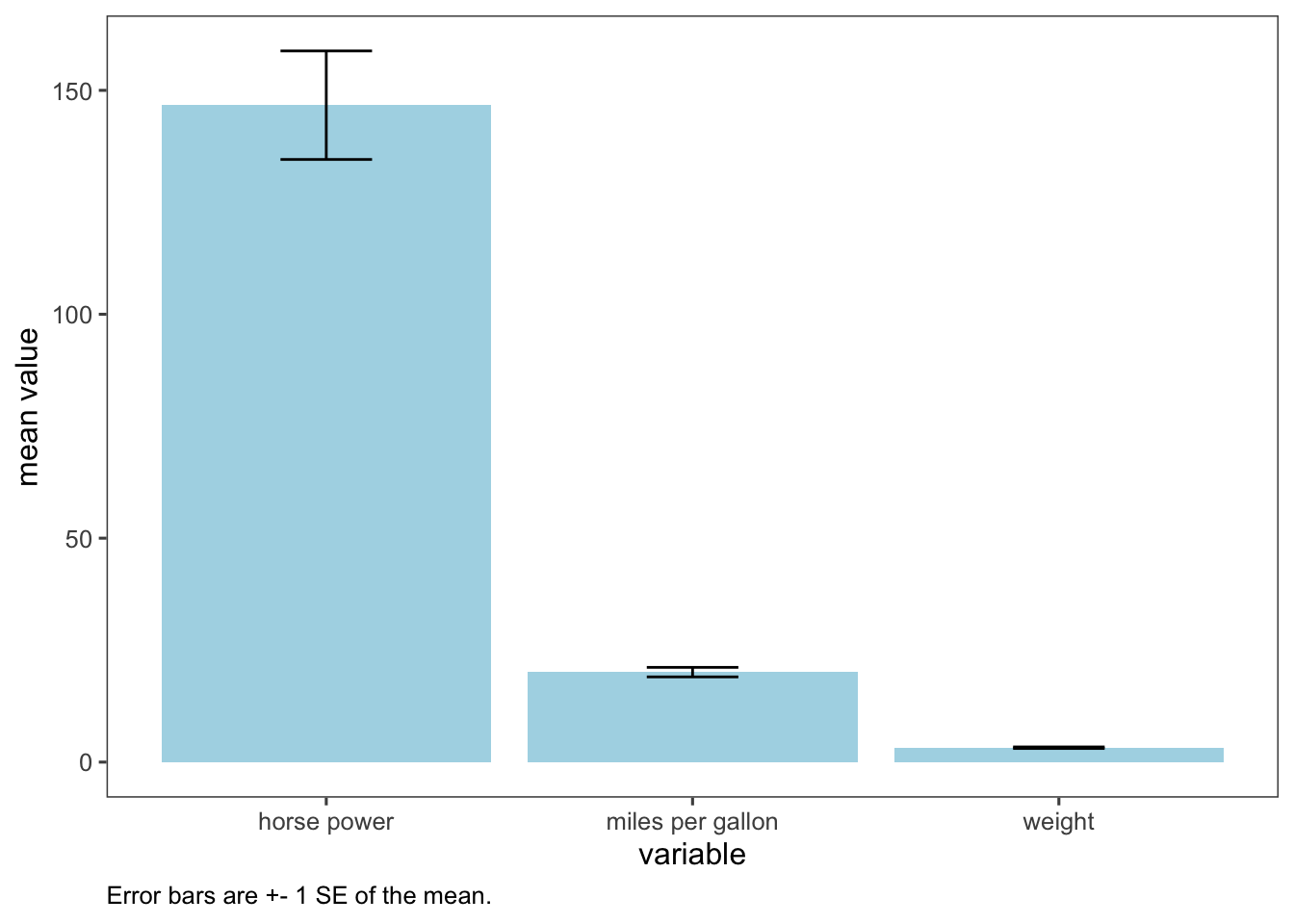
Below, I fully demonstrate how we can use our function in a pipeline that begins with purrr and ends with us using ggplot to visualize the mean and se for each of these numerical variables.
# compute summary statsmap2_dfr(list(mtcars$mpg, mtcars$hp, mtcars$wt), list("miles per gallon","horse power","weight"), sum_stat) %>%mutate(se_lower=mean-se, # get lower and upper bounds for error barsse_upper=mean+se) %>%ggplot(aes(id,mean))+geom_col(fill="lightblue")+# visualize w/ geom_colgeom_errorbar(aes(ymin=se_lower,ymax=se_upper),width=.25)+# add error barslabs(x="variable",y="mean value",caption="Error bars are +- 1 SE of the mean.")+ ggthemes::theme_few()+theme(plot.caption=element_text(hjust=0))
This plot might not be the best use of ggplot. The units of these variables are so different - for example, wt is measured in tons, so it’s very difficult to see where exactly the mean lies. So take this as an example of what you can do with purrr, when it makes sense for your research question.
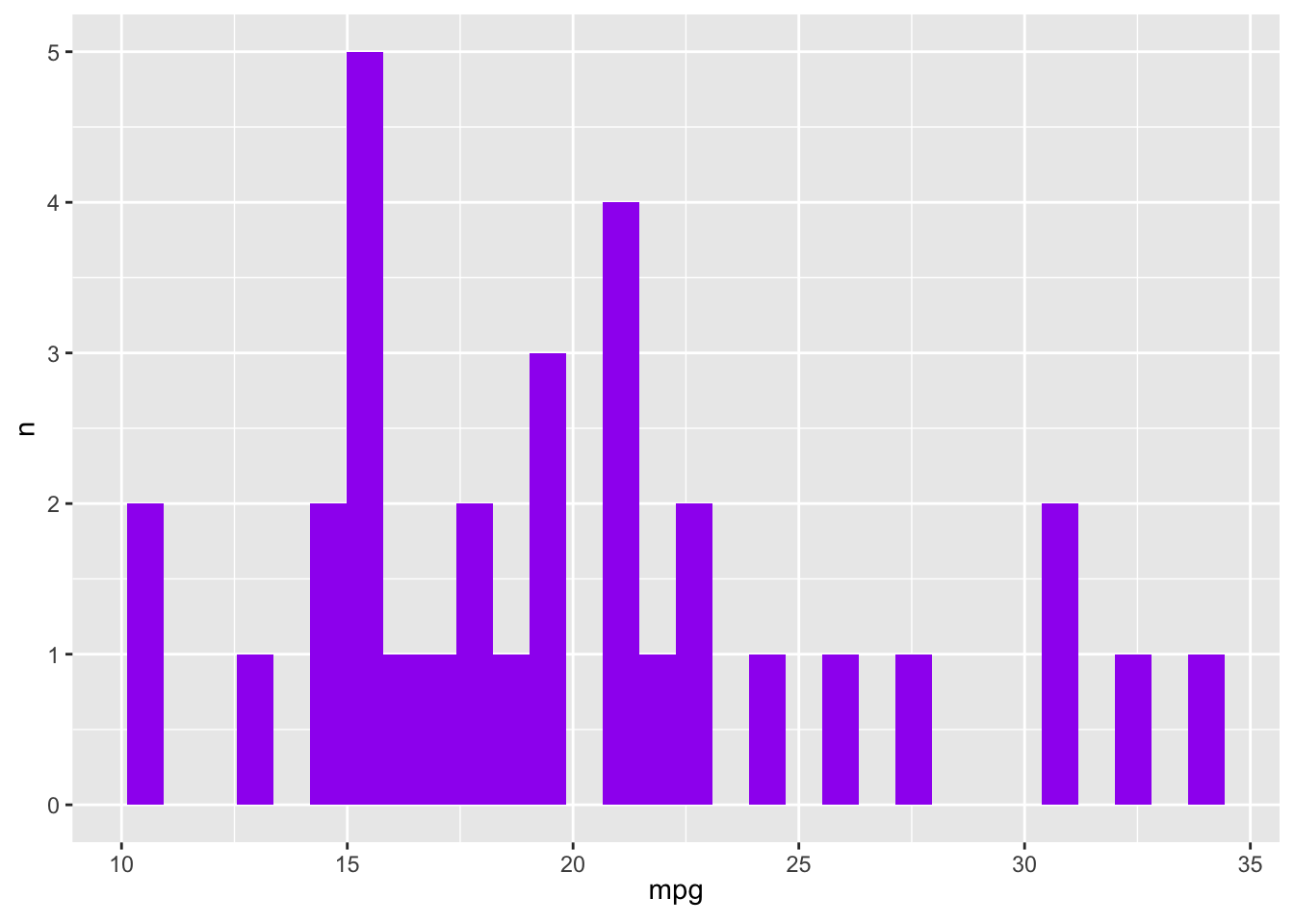
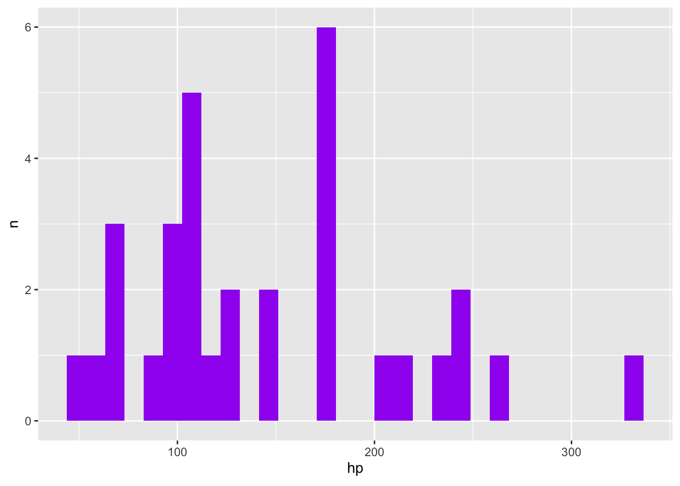
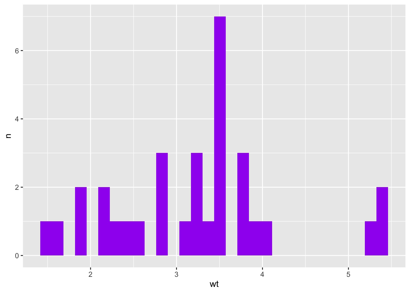
A function that plots a histogram
In Challenge 9, we made a function that creates a histogram using ggplot. Here, we use it to make multiple histograms using map().
We pass the names of the variables we want to graph to the make_my_hist() function. We use !!, or bang-bang to make sure the function works appropriately.
A function that computes counts of a categorical variable
When a variable is categorical, we typically summarise it by computing the counts (or frequencies) of each value. Base R uses the table() function to do so, but the result is of class "table", which is not always amenable to a tidyverse programmer.
The below function uses the sum() function add up the counts of each unique value in a categorical variable. A second, optional argument allows the user to compute proportions as well (also known as relative frequencies).2.
The function
# function for countingtable_data <-function(x, props=F){# get all unique values of x v <-unique(x)# using purrr, count the num of values at each unique level of x counts <-map_dbl(v, ~sum(x==.x))# combine results in a tibble res <-tibble(name=v,n=counts )# compute props if desiredif(props){ res <- res %>%mutate(prop=n/sum(n)) }return(res)}
# A tibble: 3 × 2
  name      n
  <chr> <dbl>
1 b       328
2 c       349
3 a       323
# count w/ propstable_data(vec,T)
# A tibble: 3 × 3
  name      n  prop
  <chr> <dbl> <dbl>
1 b       328 0.328
2 c       349 0.349
3 a       323 0.323
Wrapping up
The above examples are just a few ways you can use purrr to implement functional programming in R.
Footnotes
This is beyond the scope of the challenge/this course. If you’re interested, you are welcome to read more about it. The main point here is we’re using some fancy R functions to grab the column names we want from the mtcars data frame.↩︎
A user might also use the dplyr functions n() or count(), though these have drawbacks of their own↩︎
Source Code
---title: "Challenge 10 Solutions"author: "Sean Conway"description: "purrr"date: "7/6/2023"format: html: toc: true code-copy: true code-tools: truecategories: - challenge_10editor_options: chunk_output_type: console---```{r}#| label: setup#| warning: false#| message: false#| include: falselibrary(tidyverse)library(ggplot2)knitr::opts_chunk$set(echo =TRUE, warning=FALSE, message=FALSE)```## Challenge OverviewThe [purrr](https://purrr.tidyverse.org/) package is a powerful tool for functional programming. It allows the user to apply a single function across multiple objects. It can replace for loops with a more readable (and often faster) simple function call. For example, we can draw `n` random samples from 10 different distributions using a vector of 10 means. ```{r}n <-100# sample sizem <-seq(1,10) # means samps <-map(m,rnorm,n=n) samps```We can then use `map_dbl` to verify that this worked correctly by computing the mean for each sample. ```{r}samps %>%map_dbl(mean)````purrr` is tricky to learn (but beyond useful once you get a handle on it). Therefore, it's imperative that you complete the `purr` and `map` readings before attempting this challenge. ## The challenge Use `purrr` with a function to perform *some* data science task. What this task is is up to you. It could involve computing summary statistics, reading in multiple datasets, running a random process multiple times, or anything else you might need to do in your work as a data analyst. You might consider using `purrr` with a function you wrote for challenge 9. ## Solutions There are innumerable ways to use `purrr` in your coding.## Using `purrr` to perform simple computations Let's use the `map_dbl()` function to compute the mean for each of several variables. Below, we use the the `map_dbl()` function to compute the mean for multiple variables from the `mtcars` dataset (specifically weight, horsepower, and miles-per-gallon). We use `map_dbl()` because we know the result of computing the mean will be of data type `double`. This allows `purrr` to simplify the output. We also combine the variables in a `list` when passing them to `map_dbl()`. ```{r}# the datasetmtcars``````{r}map_dbl(list(mtcars$wt, mtcars$hp, mtcars$mpg),mean)```The above operation gives us a vector of means. If we use regular old `map`, the operation still works fine, but we get a list object (which can be a little more annoying to work with). ```{r}map(list(mtcars$wt, mtcars$hp, mtcars$mpg),mean)```## A function that computes multiple summary statistics I modified this function to include a required "id" value. This will allow us to use `map2_dfr()` to apply the function across multiple columns and bind the results into a single data frame, while allowing the variable itself to be identifiable. I also modified the function to compute the [standard error](https://en.wikipedia.org/wiki/Standard_error). ```{r}sum_stat <-function(x,id){ stat <-tibble(id=id,mean=mean(x,na.rm=T),median=median(x,na.rm=T),sd=sd(x,na.rm=T),se=sd/sqrt(length(x)) )return(stat)}```We'll use the `mtcars` dataset. ```{r}mtcars```In the example below, we compute the mean, median, sd, and se for `mpg` (miles per gallon), `hp` (horsepower), and `wt` (weight) in the `mtcars` dataset. We use `map2_dfr()` to do so. We need to use one of the [map2](https://purrr.tidyverse.org/reference/map2.html) variations because we need to concurrently pass the vector of numerical values and the character identifier we're using for this variable (e.g., both `mtcars$mpg` and `"mpg"`). ```{r}mtcars_stats <-map2_dfr(list(mtcars$mpg, mtcars$hp, mtcars$wt), list("mpg","hp","wt"), sum_stat)mtcars_stats```We can even use `pivot_longer()` to get a "long" format of these statistics. ```{r}mtcars_stats_long <- mtcars_stats %>%pivot_longer(c(-id))mtcars_stats_long```### A `purrr` pipeline Below, I fully demonstrate how we can use our function in a pipeline that begins with `purrr` and ends with us using `ggplot` to visualize the mean and se for each of these numerical variables. ```{r}# compute summary statsmap2_dfr(list(mtcars$mpg, mtcars$hp, mtcars$wt), list("miles per gallon","horse power","weight"), sum_stat) %>%mutate(se_lower=mean-se, # get lower and upper bounds for error barsse_upper=mean+se) %>%ggplot(aes(id,mean))+geom_col(fill="lightblue")+# visualize w/ geom_colgeom_errorbar(aes(ymin=se_lower,ymax=se_upper),width=.25)+# add error barslabs(x="variable",y="mean value",caption="Error bars are +- 1 SE of the mean.")+ ggthemes::theme_few()+theme(plot.caption=element_text(hjust=0))```This plot might not be the best use of `ggplot`. The units of these variables are so different - for example, `wt` is measured in tons, so it's very difficult to see where exactly the mean lies. So take this as an example of what you *can* do with `purrr`, when it makes sense for your research question. ## A function that plots a histogram In Challenge 9, we made a function that creates a histogram using ggplot. Here, we use it to make multiple histograms using `map()`. We have to modify the function using [defusion](https://rlang.r-lib.org/reference/topic-defuse.html)^[This is beyond the scope of the challenge/this course. If you're interested, you are welcome to read more about it. The main point here is we're using some fancy `R` functions to grab the column names we want from the `mtcars` data frame.]. ```{r}make_my_hist <-function(dat, colname, fill="purple", xlab="x", ylab="n"){ colname <- rlang::ensym(colname) dat %>%ggplot(aes({{colname}}))+geom_histogram(fill=fill)+labs(x=colname,y=ylab)}```### Making the histograms We pass the names of the variables we want to graph to the `make_my_hist()` function. We use `!!`, or [bang-bang](https://www.r-bloggers.com/2019/07/bang-bang-how-to-program-with-dplyr/) to make sure the function works appropriately. ```{r}map(c("mpg", "hp", "wt"), ~make_my_hist(dat=mtcars, colname=!!.x))```## A function that computes counts of a categorical variable When a variable is categorical, we typically summarise it by computing the counts (or frequencies) of each value. Base `R` uses the `table()` function to do so, but the result is of class `"table"`, which is not always amenable to a tidyverse programmer. The below function uses the `sum()` function add up the counts of each unique value in a categorical variable. A second, optional argument allows the user to compute proportions as well (also known as relative frequencies).^[A user might also use the `dplyr` functions `n()` or `count()`, though these have drawbacks of their own]. ### The function ```{r}# function for countingtable_data <-function(x, props=F){# get all unique values of x v <-unique(x)# using purrr, count the num of values at each unique level of x counts <-map_dbl(v, ~sum(x==.x))# combine results in a tibble res <-tibble(name=v,n=counts )# compute props if desiredif(props){ res <- res %>%mutate(prop=n/sum(n)) }return(res)}```### Using the functions ```{r}# randomly sampled vectorvec <-sample(c("a","b","c"),size=1000,replace=T)head(vec)``````{r}# count w/o propstable_data(vec)# count w/ propstable_data(vec,T)```## Wrapping up The above examples are just a few ways you can use `purrr` to implement functional programming in `R`.