Challenge 1 Submission

Reading in data and creating a post

Code

library(tidyverse)

knitr::opts_chunk$set(echo = TRUE, warning=FALSE, message=FALSE)

Challenge Overview

Today’s challenge is to

1. read in a dataset, and

2. describe the dataset using both words and any supporting information (e.g., tables, etc)

Read in the Data

Read in one (or more) of the following data sets, using the correct R package and command.

• railroad_2012_clean_county.csv ⭐
• birds.csv ⭐⭐
• FAOstat*.csv ⭐⭐
• wild_bird_data.xlsx ⭐⭐⭐
• StateCounty2012.xls ⭐⭐⭐⭐

Find the _data folder, located inside the posts folder. Then you can read in the data, using either one of the readr standard tidy read commands, or a specialized package such as readxl.

Code

data_railroad <- read_csv("_data/railroad_2012_clean_county.csv")

Add any comments or documentation as needed. More challenging data sets may require additional code chunks and documentation.

Describe the data

Using a combination of words and results of R commands, can you provide a high level description of the data? Describe as efficiently as possible where/how the data was (likely) gathered, indicate the cases and variables (both the interpretation and any details you deem useful to the reader to fully understand your chosen data).

we choose - railroad_2012_clean_county.csv ⭐

Code

data <- read.csv("_data/railroad_2012_clean_county.csv")
head(data)

Code

summary(data)

    state              county          total_employees  
 Length:2930        Length:2930        Min.   :   1.00  
 Class :character   Class :character   1st Qu.:   7.00  
 Mode  :character   Mode  :character   Median :  21.00  
                                       Mean   :  87.18  
                                       3rd Qu.:  65.00  
                                       Max.   :8207.00  

The summary indicates that the dataset comprises 2930 observations each with three variables: state, county, and total_employees.

state and county are both of character class, indicating that they hold textual information. They represent the US states and counties, respectively.

total_employees is of integer class and represents the total number of employees in each county. The key statistics of this variable are:

Minimum: 1 - This is the smallest number of total employees in a county within the dataset. 1st Quartile (25th percentile): 7 - 25% of the counties have 7 or fewer employees. Median (50th percentile): 21 - Half of the counties have 21 or fewer employees. Mean: 87.18 - On average, a county has approximately 87 employees. 3rd Quartile (75th percentile): 65 - 75% of the counties have 65 or fewer employees. Maximum: 8207 - This is the largest number of total employees in a county within the datase

Code

#National total number of employees
sum(data$total_employees)

[1] 255432

Code

# Total number of employees in each state
aggregate(total_employees ~ state, data = data, sum)

The above two tables are the total number of employees in the country and the total number of employees in each state. We can see that most of the employees are located in the east.

Code

library(ggplot2)

# Histogram of the total number of employees in each state
state_summary <- aggregate(total_employees ~ state, data = data, sum)
ggplot(state_summary, aes(x = state, y = total_employees)) +
  geom_bar(stat = "identity") +
  theme(axis.text.x = element_text(angle = 90, hjust = 1)) +
  labs(x = "State", y = "Total Employees", title = "Total Employees by State")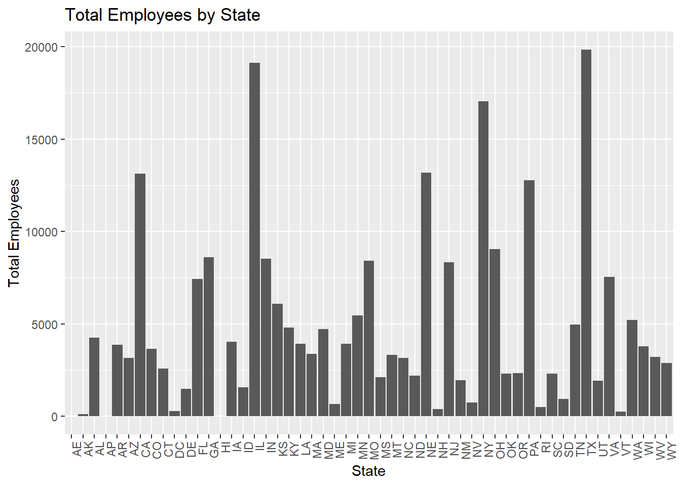

This is a histogram visualization of the total number of employees by state, which is the same as the above graph to analyze. The visualization chart can let us know more clearly the distribution of employees in different regions. Among them, TN, NY, and IL have the largest number of employees, and AE, VT, and CD have the least number of employees