Code
library(tidyverse)

knitr::opts_chunk$set(echo = TRUE, warning=FALSE, message=FALSE)Shreya Varma
July 4, 2023
Today’s challenge is to
Read in one (or more) of the following data sets, available in the posts/_data folder, using the correct R package and command.
Add any comments or documentation as needed. More challenging data may require additional code chunks and documentation.
Using a combination of words and results of R commands, can you provide a high level description of the data? Describe as efficiently as possible where/how the data was (likely) gathered, indicate the cases and variables (both the interpretation and any details you deem useful to the reader to fully understand your chosen data).
I will be using the Hotel Bookings dataset for my Homework. I have imported it using the read_csv() function and will use the glimpse() function the see the columns it has. On a high level it seems to have the information of hotel type and its customer data like arrival departure information, number of people, their booking details, payment type and reservation details. The data has 119,390 rows and 32 columns and seems to be captured from different hotels between 2015 to 2015 when people checked in and out. To get more insights I will use the summary() function.
# A tibble: 119,390 × 32
hotel is_canceled lead_time arrival_date_year arrival_date_month
<chr> <dbl> <dbl> <dbl> <chr>
1 Resort Hotel 0 342 2015 July
2 Resort Hotel 0 737 2015 July
3 Resort Hotel 0 7 2015 July
4 Resort Hotel 0 13 2015 July
5 Resort Hotel 0 14 2015 July
6 Resort Hotel 0 14 2015 July
7 Resort Hotel 0 0 2015 July
8 Resort Hotel 0 9 2015 July
9 Resort Hotel 1 85 2015 July
10 Resort Hotel 1 75 2015 July
# ℹ 119,380 more rows
# ℹ 27 more variables: arrival_date_week_number <dbl>,
# arrival_date_day_of_month <dbl>, stays_in_weekend_nights <dbl>,
# stays_in_week_nights <dbl>, adults <dbl>, children <dbl>, babies <dbl>,
# meal <chr>, country <chr>, market_segment <chr>,
# distribution_channel <chr>, is_repeated_guest <dbl>,
# previous_cancellations <dbl>, previous_bookings_not_canceled <dbl>, …Rows: 119,390
Columns: 32
$ hotel <chr> "Resort Hotel", "Resort Hotel", "Resort…
$ is_canceled <dbl> 0, 0, 0, 0, 0, 0, 0, 0, 1, 1, 1, 0, 0, …
$ lead_time <dbl> 342, 737, 7, 13, 14, 14, 0, 9, 85, 75, …
$ arrival_date_year <dbl> 2015, 2015, 2015, 2015, 2015, 2015, 201…
$ arrival_date_month <chr> "July", "July", "July", "July", "July",…
$ arrival_date_week_number <dbl> 27, 27, 27, 27, 27, 27, 27, 27, 27, 27,…
$ arrival_date_day_of_month <dbl> 1, 1, 1, 1, 1, 1, 1, 1, 1, 1, 1, 1, 1, …
$ stays_in_weekend_nights <dbl> 0, 0, 0, 0, 0, 0, 0, 0, 0, 0, 0, 0, 0, …
$ stays_in_week_nights <dbl> 0, 0, 1, 1, 2, 2, 2, 2, 3, 3, 4, 4, 4, …
$ adults <dbl> 2, 2, 1, 1, 2, 2, 2, 2, 2, 2, 2, 2, 2, …
$ children <dbl> 0, 0, 0, 0, 0, 0, 0, 0, 0, 0, 0, 0, 0, …
$ babies <dbl> 0, 0, 0, 0, 0, 0, 0, 0, 0, 0, 0, 0, 0, …
$ meal <chr> "BB", "BB", "BB", "BB", "BB", "BB", "BB…
$ country <chr> "PRT", "PRT", "GBR", "GBR", "GBR", "GBR…
$ market_segment <chr> "Direct", "Direct", "Direct", "Corporat…
$ distribution_channel <chr> "Direct", "Direct", "Direct", "Corporat…
$ is_repeated_guest <dbl> 0, 0, 0, 0, 0, 0, 0, 0, 0, 0, 0, 0, 0, …
$ previous_cancellations <dbl> 0, 0, 0, 0, 0, 0, 0, 0, 0, 0, 0, 0, 0, …
$ previous_bookings_not_canceled <dbl> 0, 0, 0, 0, 0, 0, 0, 0, 0, 0, 0, 0, 0, …
$ reserved_room_type <chr> "C", "C", "A", "A", "A", "A", "C", "C",…
$ assigned_room_type <chr> "C", "C", "C", "A", "A", "A", "C", "C",…
$ booking_changes <dbl> 3, 4, 0, 0, 0, 0, 0, 0, 0, 0, 0, 0, 0, …
$ deposit_type <chr> "No Deposit", "No Deposit", "No Deposit…
$ agent <chr> "NULL", "NULL", "NULL", "304", "240", "…
$ company <chr> "NULL", "NULL", "NULL", "NULL", "NULL",…
$ days_in_waiting_list <dbl> 0, 0, 0, 0, 0, 0, 0, 0, 0, 0, 0, 0, 0, …
$ customer_type <chr> "Transient", "Transient", "Transient", …
$ adr <dbl> 0.00, 0.00, 75.00, 75.00, 98.00, 98.00,…
$ required_car_parking_spaces <dbl> 0, 0, 0, 0, 0, 0, 0, 0, 0, 0, 0, 0, 0, …
$ total_of_special_requests <dbl> 0, 0, 0, 0, 1, 1, 0, 1, 1, 0, 0, 0, 3, …
$ reservation_status <chr> "Check-Out", "Check-Out", "Check-Out", …
$ reservation_status_date <date> 2015-07-01, 2015-07-01, 2015-07-02, 20…Conduct some exploratory data analysis, using dplyr commands such as group_by(), select(), filter(), and summarise(). Find the central tendency (mean, median, mode) and dispersion (standard deviation, mix/max/quantile) for different subgroups within the data set.
hotel is_canceled lead_time arrival_date_year
Length:119390 Min. :0.0000 Min. : 0 Min. :2015
Class :character 1st Qu.:0.0000 1st Qu.: 18 1st Qu.:2016
Mode :character Median :0.0000 Median : 69 Median :2016
Mean :0.3704 Mean :104 Mean :2016
3rd Qu.:1.0000 3rd Qu.:160 3rd Qu.:2017
Max. :1.0000 Max. :737 Max. :2017
arrival_date_month arrival_date_week_number arrival_date_day_of_month
Length:119390 Min. : 1.00 Min. : 1.0
Class :character 1st Qu.:16.00 1st Qu.: 8.0
Mode :character Median :28.00 Median :16.0
Mean :27.17 Mean :15.8
3rd Qu.:38.00 3rd Qu.:23.0
Max. :53.00 Max. :31.0
stays_in_weekend_nights stays_in_week_nights adults
Min. : 0.0000 Min. : 0.0 Min. : 0.000
1st Qu.: 0.0000 1st Qu.: 1.0 1st Qu.: 2.000
Median : 1.0000 Median : 2.0 Median : 2.000
Mean : 0.9276 Mean : 2.5 Mean : 1.856
3rd Qu.: 2.0000 3rd Qu.: 3.0 3rd Qu.: 2.000
Max. :19.0000 Max. :50.0 Max. :55.000
children babies meal country
Min. : 0.0000 Min. : 0.000000 Length:119390 Length:119390
1st Qu.: 0.0000 1st Qu.: 0.000000 Class :character Class :character
Median : 0.0000 Median : 0.000000 Mode :character Mode :character
Mean : 0.1039 Mean : 0.007949
3rd Qu.: 0.0000 3rd Qu.: 0.000000
Max. :10.0000 Max. :10.000000
NA's :4
market_segment distribution_channel is_repeated_guest
Length:119390 Length:119390 Min. :0.00000
Class :character Class :character 1st Qu.:0.00000
Mode :character Mode :character Median :0.00000
Mean :0.03191
3rd Qu.:0.00000
Max. :1.00000
previous_cancellations previous_bookings_not_canceled reserved_room_type
Min. : 0.00000 Min. : 0.0000 Length:119390
1st Qu.: 0.00000 1st Qu.: 0.0000 Class :character
Median : 0.00000 Median : 0.0000 Mode :character
Mean : 0.08712 Mean : 0.1371
3rd Qu.: 0.00000 3rd Qu.: 0.0000
Max. :26.00000 Max. :72.0000
assigned_room_type booking_changes deposit_type agent
Length:119390 Min. : 0.0000 Length:119390 Length:119390
Class :character 1st Qu.: 0.0000 Class :character Class :character
Mode :character Median : 0.0000 Mode :character Mode :character
Mean : 0.2211
3rd Qu.: 0.0000
Max. :21.0000
company days_in_waiting_list customer_type adr
Length:119390 Min. : 0.000 Length:119390 Min. : -6.38
Class :character 1st Qu.: 0.000 Class :character 1st Qu.: 69.29
Mode :character Median : 0.000 Mode :character Median : 94.58
Mean : 2.321 Mean : 101.83
3rd Qu.: 0.000 3rd Qu.: 126.00
Max. :391.000 Max. :5400.00
required_car_parking_spaces total_of_special_requests reservation_status
Min. :0.00000 Min. :0.0000 Length:119390
1st Qu.:0.00000 1st Qu.:0.0000 Class :character
Median :0.00000 Median :0.0000 Mode :character
Mean :0.06252 Mean :0.5714
3rd Qu.:0.00000 3rd Qu.:1.0000
Max. :8.00000 Max. :5.0000
reservation_status_date
Min. :2014-10-17
1st Qu.:2016-02-01
Median :2016-08-07
Mean :2016-07-30
3rd Qu.:2017-02-08
Max. :2017-09-14
Error in eval(expr, envir, enclos): object 'lead_time_stats' not found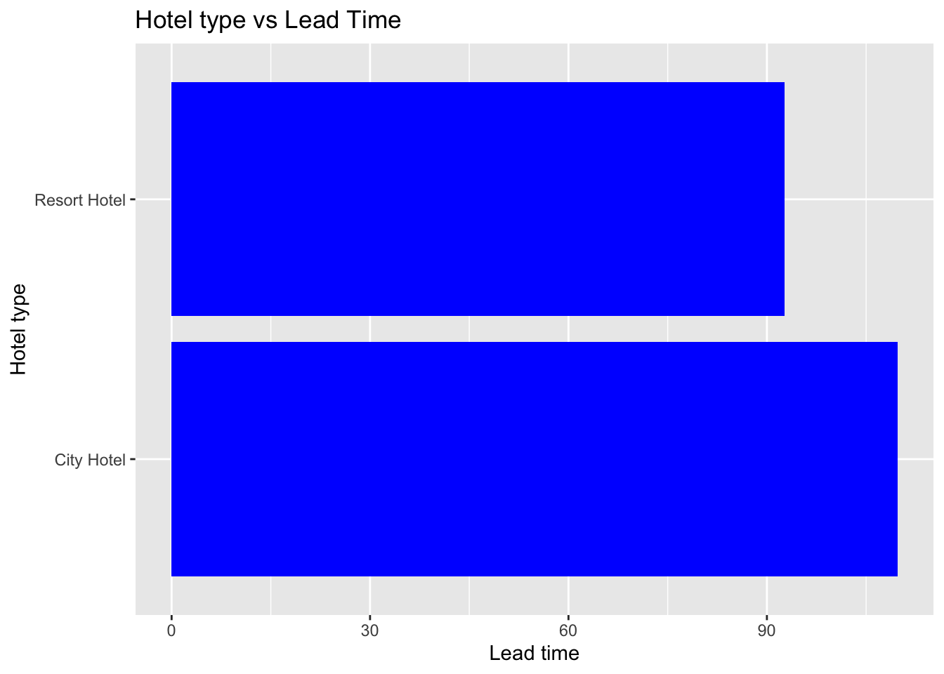
is_categorical <- class(hotel_bookings$is_canceled) == "factor" || is.character(hotel_bookings$is_canceled)
# Convert to categorical if not already
if (!is_categorical) {
hotel_bookings$is_canceled <- as.factor(hotel_bookings$is_canceled)
}
active_booking <- hotel_bookings %>%
filter(deposit_type== 'Non Refund') %>%
select(hotel, is_canceled)
hotel_bookings%>%
ggplot(aes(x=hotel,fill=is_canceled)) + geom_bar()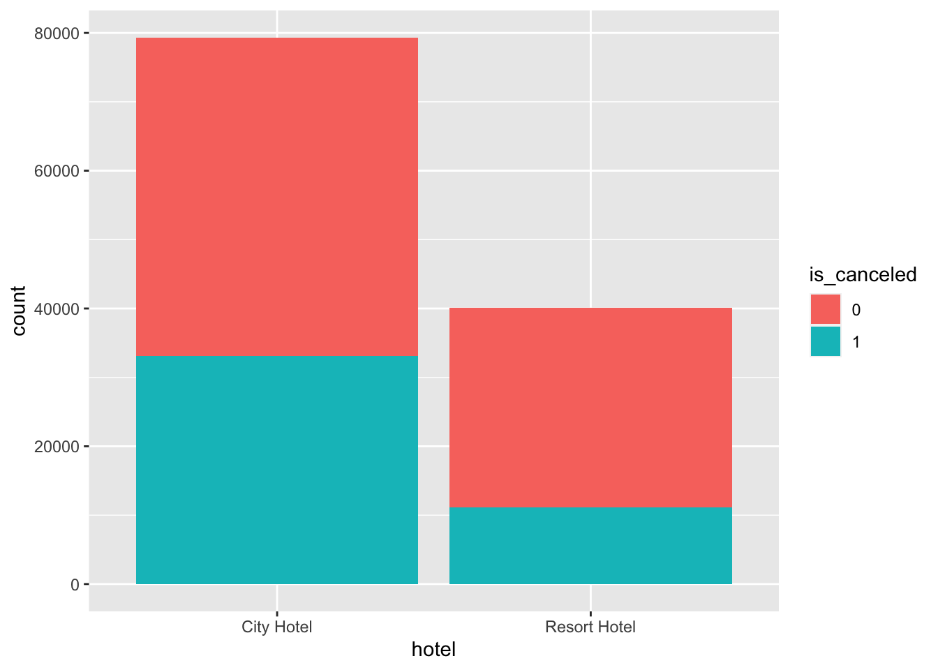
Be sure to explain why you choose a specific group. Comment on the interpretation of any interesting differences between groups that you uncover. This section can be integrated with the exploratory data analysis, just be sure it is included.
From the summary we can see that mean lead time is 104 days which means that people book their stays approximately 3 to 3.5 months in advance. We can also check if the lead time is higher for Resort hotels vs for City hotels. My hypothesis is that it should be higher for Resort hotels since people book their vacations in advance but City hotels can be booked due to office work or immediate need basis too.
We can see that my hypothesis is not correct and the lead time for City hotels is slightly higher infact. This could also be due to the fact that we have more data of City hotels than Resort hotel. Almost twice. This could skew the lead time thus we cannot say for sure about lead time or analysis related to Hotel type.
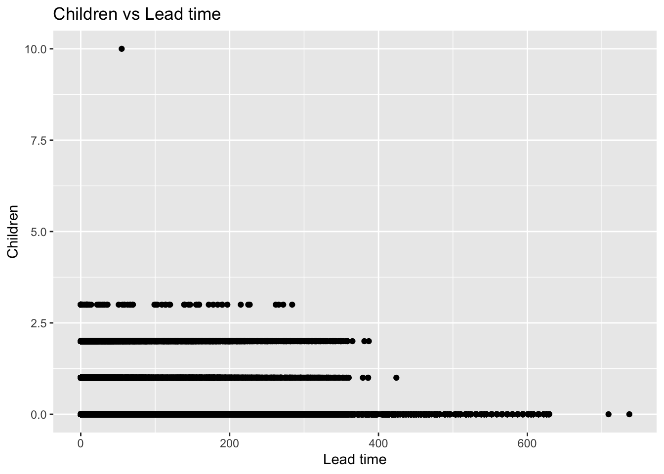
Instead I checked if people with children have a higher lead time. Thus I created the plot of children vs lead time. However we can see that people with 0 children have higher lead time. Thus the hypothesis is false.
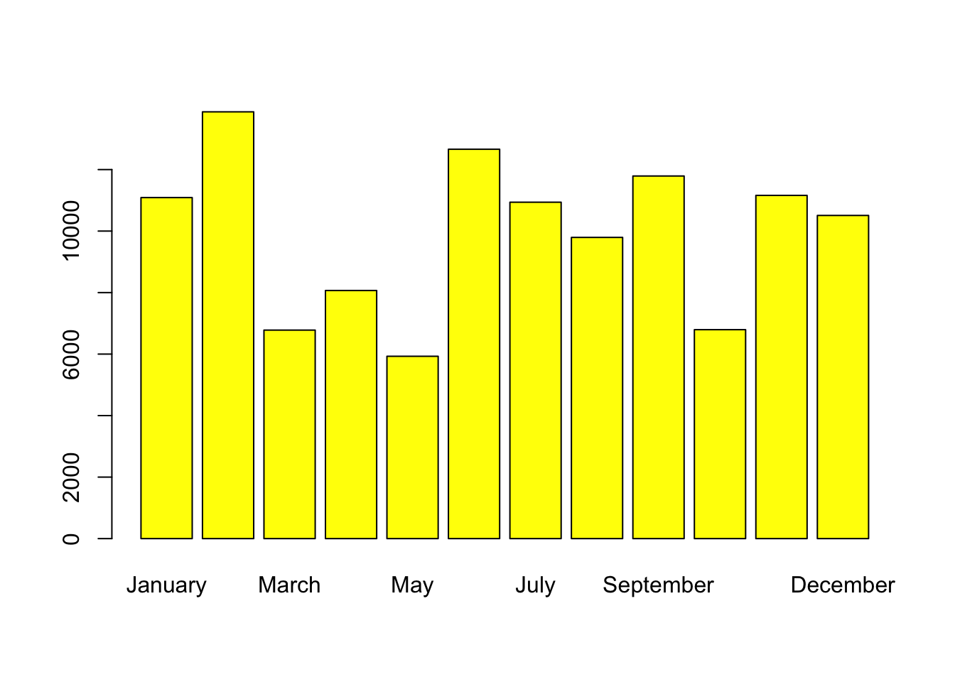
I also checked with arrival month frequency and it looks like February was the highest frequency month.
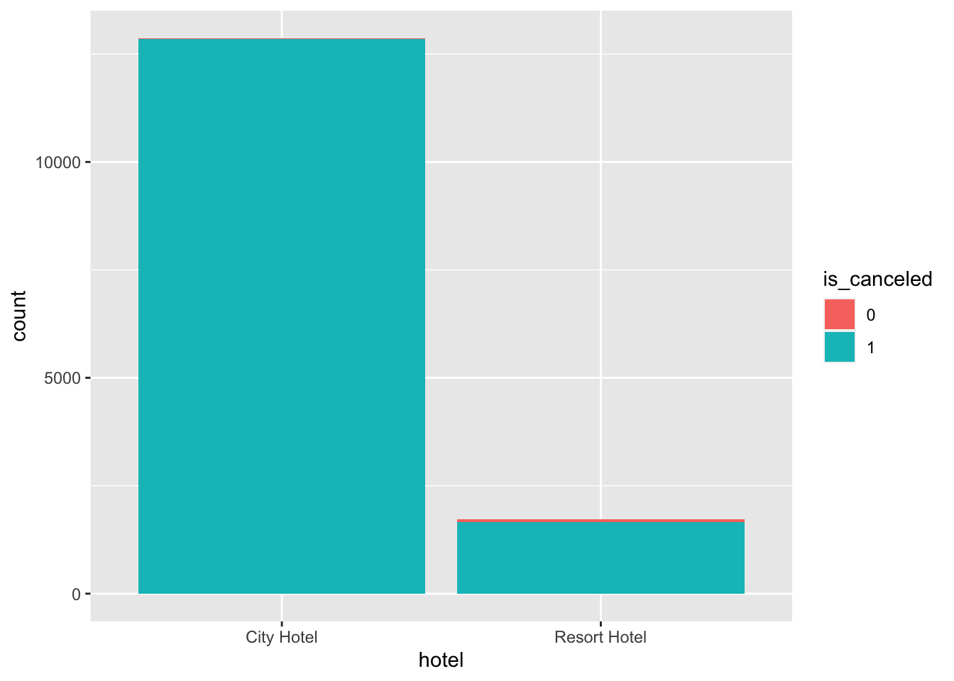
We can also see that people do make cancellations for deposit type ‘Non Refund’ very often too. Thus we cannot say that a Non refundable booking will result in no cancellations.
---
title: "Challenge 2 Solution"
author: "Shreya Varma"
description: "Data wrangling: using group() and summarise()"
date: "7/4/2023"
format:
html:
toc: true
code-fold: true
code-copy: true
code-tools: true
categories:
- challenge_2
- railroads
- faostat
- hotel_bookings
---
```{r}
#| label: setup
#| warning: false
#| message: false
library(tidyverse)
knitr::opts_chunk$set(echo = TRUE, warning=FALSE, message=FALSE)
```
## Challenge Overview
Today's challenge is to
1) read in a data set, and describe the data using both words and any supporting information (e.g., tables, etc)
2) provide summary statistics for different interesting groups within the data, and interpret those statistics
## Read in the Data
Read in one (or more) of the following data sets, available in the `posts/_data` folder, using the correct R package and command.
- railroad\*.csv or StateCounty2012.xls ⭐
- FAOstat\*.csv or birds.csv ⭐⭐⭐
- hotel_bookings.csv ⭐⭐⭐⭐
```{r}
```
Add any comments or documentation as needed. More challenging data may require additional code chunks and documentation.
## Describe the data
Using a combination of words and results of R commands, can you provide a high level description of the data? Describe as efficiently as possible where/how the data was (likely) gathered, indicate the cases and variables (both the interpretation and any details you deem useful to the reader to fully understand your chosen data).
I will be using the Hotel Bookings dataset for my Homework. I have imported it using the read_csv() function and will use the glimpse() function the see the columns it has. On a high level it seems to have the information of hotel type and its customer data like arrival departure information, number of people, their booking details, payment type and reservation details. The data has 119,390 rows and 32 columns and seems to be captured from different hotels between 2015 to 2015 when people checked in and out. To get more insights I will use the summary() function.
```{r}
hotel_bookings <- read_csv("_data/hotel_bookings.csv")
hotel_bookings
glimpse(hotel_bookings)
```
## Provide Grouped Summary Statistics
Conduct some exploratory data analysis, using dplyr commands such as `group_by()`, `select()`, `filter()`, and `summarise()`. Find the central tendency (mean, median, mode) and dispersion (standard deviation, mix/max/quantile) for different subgroups within the data set.
```{r}
summary(hotel_bookings)
lead_time_summary <- hotel_bookings %>%
  group_by(hotel) %>%
  summarize('mean_lead_time' = mean(lead_time), 'max_lead_time' = max(lead_time), 'min_lead_time' = min(lead_time))

lead_time_stats
ggplot(data = lead_time_summary, aes(x = mean_lead_time, y = hotel)) +
  # Specify the type of plot and customize it as needed
  geom_col(fill = "blue") +
  labs(title = "Hotel type vs Lead Time", x = "Lead time", y = "Hotel type")
ggplot(data = hotel_bookings, aes(x = lead_time, y = children)) +
  geom_point() +
  labs(title = "Children vs Lead time", x = "Lead time", y = "Children")
month_counts <- table(hotel_bookings$arrival_date_month)
barplot(month_counts, names.arg = month.name, col = 'yellow')
is_categorical <- class(hotel_bookings$is_canceled) == "factor" || is.character(hotel_bookings$is_canceled)

# Convert to categorical if not already
if (!is_categorical) {
  hotel_bookings$is_canceled <- as.factor(hotel_bookings$is_canceled)
}


active_booking <- hotel_bookings %>%
  filter(deposit_type== 'Non Refund') %>%
  select(hotel, is_canceled)

hotel_bookings%>%
  ggplot(aes(x=hotel,fill=is_canceled)) + geom_bar()
active_booking%>%
  ggplot(aes(x=hotel,fill=is_canceled)) + geom_bar()
```
### Explain and Interpret
Be sure to explain why you choose a specific group. Comment on the interpretation of any interesting differences between groups that you uncover. This section can be integrated with the exploratory data analysis, just be sure it is included.
From the summary we can see that mean lead time is 104 days which means that people book their stays approximately 3 to 3.5 months in advance. We can also check if the lead time is higher for Resort hotels vs for City hotels. My hypothesis is that it should be higher for Resort hotels since people book their vacations in advance but City hotels can be booked due to office work or immediate need basis too.
We can see that my hypothesis is not correct and the lead time for City hotels is slightly higher infact. This could also be due to the fact that we have more data of City hotels than Resort hotel. Almost twice. This could skew the lead time thus we cannot say for sure about lead time or analysis related to Hotel type.
Instead I checked if people with children have a higher lead time. Thus I created the plot of children vs lead time. However we can see that people with 0 children have higher lead time. Thus the hypothesis is false.
I also checked with arrival month frequency and it looks like February was the highest frequency month.
We can also see that people do make cancellations for deposit type 'Non Refund' very often too. Thus we cannot say that a Non refundable booking will result in no cancellations.