Challenge 2 - Hotel Bookings

challenge_2

hotel_bookings

srujan_kagitala

Data wrangling: using group() and summarise()

Author

Srujan Kagitala

Published

June 26, 2023

Code

library(tidyverse)

knitr::opts_chunk$set(echo = TRUE, warning=FALSE, message=FALSE)

Challenge Overview

Today’s challenge is to

read in a data set, and describe the data using both words and any supporting information (e.g., tables, etc)
provide summary statistics for different interesting groups within the data, and interpret those statistics

Read in the Data

Read in one (or more) of the following data sets, available in the posts/_data folder, using the correct R package and command.

hotel_bookings.csv ⭐⭐⭐⭐

Code

booking_data <- read.csv("_data/hotel_bookings.csv")
head(booking_data)

         hotel is_canceled lead_time arrival_date_year arrival_date_month
1 Resort Hotel           0       342              2015               July
2 Resort Hotel           0       737              2015               July
3 Resort Hotel           0         7              2015               July
4 Resort Hotel           0        13              2015               July
5 Resort Hotel           0        14              2015               July
6 Resort Hotel           0        14              2015               July
  arrival_date_week_number arrival_date_day_of_month stays_in_weekend_nights
1                       27                         1                       0
2                       27                         1                       0
3                       27                         1                       0
4                       27                         1                       0
5                       27                         1                       0
6                       27                         1                       0
  stays_in_week_nights adults children babies meal country market_segment
1                    0      2        0      0   BB     PRT         Direct
2                    0      2        0      0   BB     PRT         Direct
3                    1      1        0      0   BB     GBR         Direct
4                    1      1        0      0   BB     GBR      Corporate
5                    2      2        0      0   BB     GBR      Online TA
6                    2      2        0      0   BB     GBR      Online TA
  distribution_channel is_repeated_guest previous_cancellations
1               Direct                 0                      0
2               Direct                 0                      0
3               Direct                 0                      0
4            Corporate                 0                      0
5                TA/TO                 0                      0
6                TA/TO                 0                      0
  previous_bookings_not_canceled reserved_room_type assigned_room_type
1                              0                  C                  C
2                              0                  C                  C
3                              0                  A                  C
4                              0                  A                  A
5                              0                  A                  A
6                              0                  A                  A
  booking_changes deposit_type agent company days_in_waiting_list customer_type
1               3   No Deposit  NULL    NULL                    0     Transient
2               4   No Deposit  NULL    NULL                    0     Transient
3               0   No Deposit  NULL    NULL                    0     Transient
4               0   No Deposit   304    NULL                    0     Transient
5               0   No Deposit   240    NULL                    0     Transient
6               0   No Deposit   240    NULL                    0     Transient
  adr required_car_parking_spaces total_of_special_requests reservation_status
1   0                           0                         0          Check-Out
2   0                           0                         0          Check-Out
3  75                           0                         0          Check-Out
4  75                           0                         0          Check-Out
5  98                           0                         1          Check-Out
6  98                           0                         1          Check-Out
  reservation_status_date
1              2015-07-01
2              2015-07-01
3              2015-07-02
4              2015-07-02
5              2015-07-03
6              2015-07-03

Add any comments or documentation as needed. More challenging data may require additional code chunks and documentation.

Describe the data

Using a combination of words and results of R commands, can you provide a high level description of the data? Describe as efficiently as possible where/how the data was (likely) gathered, indicate the cases and variables (both the interpretation and any details you deem useful to the reader to fully understand your chosen data).

Code

#Number of bookings per hotel.
no_bookings_by_hotel <- booking_data %>%
  group_by(hotel) %>%
  summarise(count = n())

This data set contains booking data of City Hotel, Resort Hotel. It contains 119390 bookings information. 79330 and 40060 observations are respectively captured from City Hotel and Resort Hotel. The information available per booking are hotel, is_canceled, lead_time, arrival_date_year, arrival_date_month, arrival_date_week_number, arrival_date_day_of_month, stays_in_weekend_nights, stays_in_week_nights, adults, children, babies, meal, country, market_segment, distribution_channel, is_repeated_guest, previous_cancellations, previous_bookings_not_canceled, reserved_room_type, assigned_room_type, booking_changes, deposit_type, agent, company, days_in_waiting_list, customer_type, adr, required_car_parking_spaces, total_of_special_requests, reservation_status, reservation_status_date.

Provide Grouped Summary Statistics

Conduct some exploratory data analysis, using dplyr commands such as group_by(), select(), filter(), and summarise(). Find the central tendency (mean, median, mode) and dispersion (standard deviation, mix/max/quantile) for different subgroups within the data set.

Code

# Number of bookings cancelled versus not cancelled 
# per hotel across years 
(hotel_booking_by_year <- booking_data %>%
  group_by(hotel, arrival_date_year, is_canceled) %>%
  summarise(no_bookings = n()))

# A tibble: 12 × 4
# Groups:   hotel, arrival_date_year [6]
   hotel        arrival_date_year is_canceled no_bookings
   <chr>                    <int>       <int>       <int>
 1 City Hotel                2015           0        7678
 2 City Hotel                2015           1        6004
 3 City Hotel                2016           0       22733
 4 City Hotel                2016           1       15407
 5 City Hotel                2017           0       15817
 6 City Hotel                2017           1       11691
 7 Resort Hotel              2015           0        6176
 8 Resort Hotel              2015           1        2138
 9 Resort Hotel              2016           0       13637
10 Resort Hotel              2016           1        4930
11 Resort Hotel              2017           0        9125
12 Resort Hotel              2017           1        4054

Code

total_hotel_bookings_by_year <- hotel_booking_by_year %>%
  group_by(hotel, arrival_date_year) %>%
  summarise(no_bookings = sum(no_bookings))

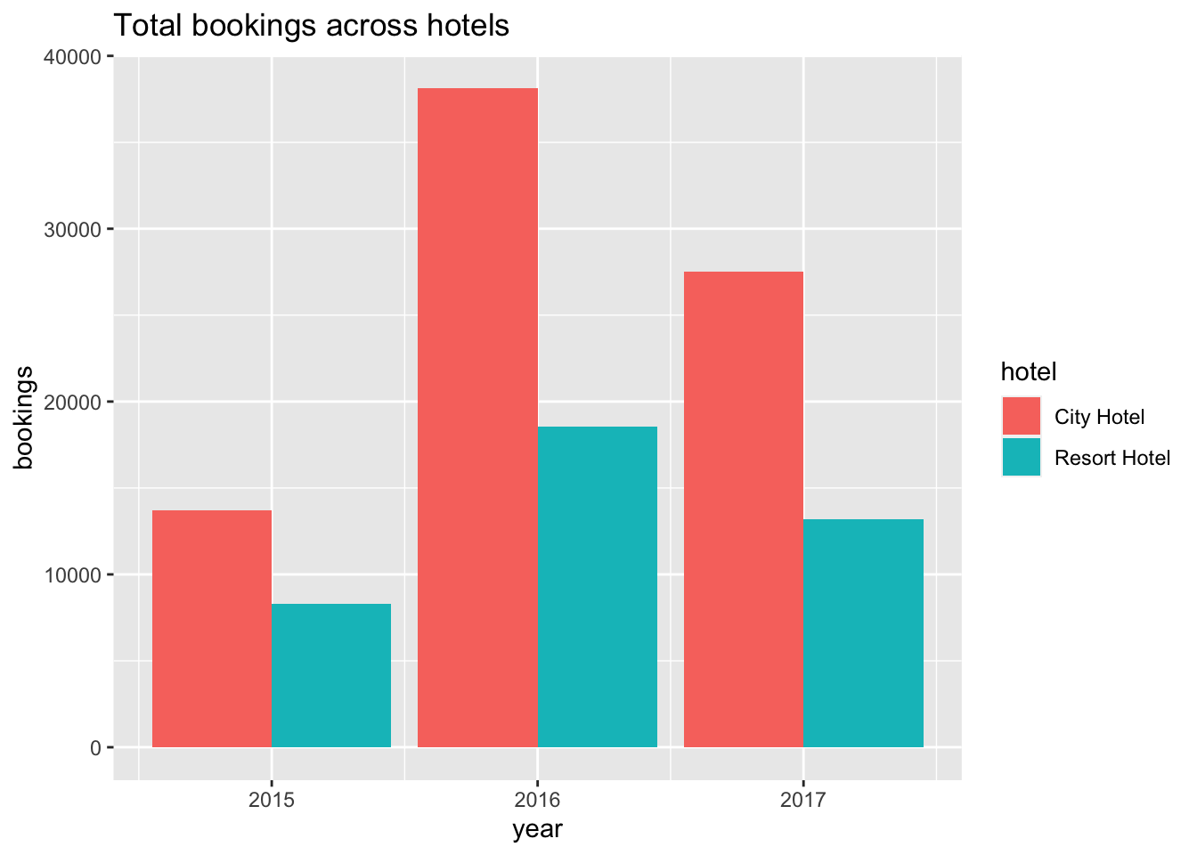
ggplot(data = total_hotel_bookings_by_year, aes(x= arrival_date_year, y=no_bookings)) +
  geom_bar(stat = "identity", mapping = aes(fill = hotel), position = "dodge") +
  ggtitle("Total bookings across hotels") +
  ylab("bookings") +
  xlab("year")

Code

cancelled_bookings_by_year <- hotel_booking_by_year %>% 
  filter(is_canceled == 1) %>%
  select(hotel, arrival_date_year, no_bookings)

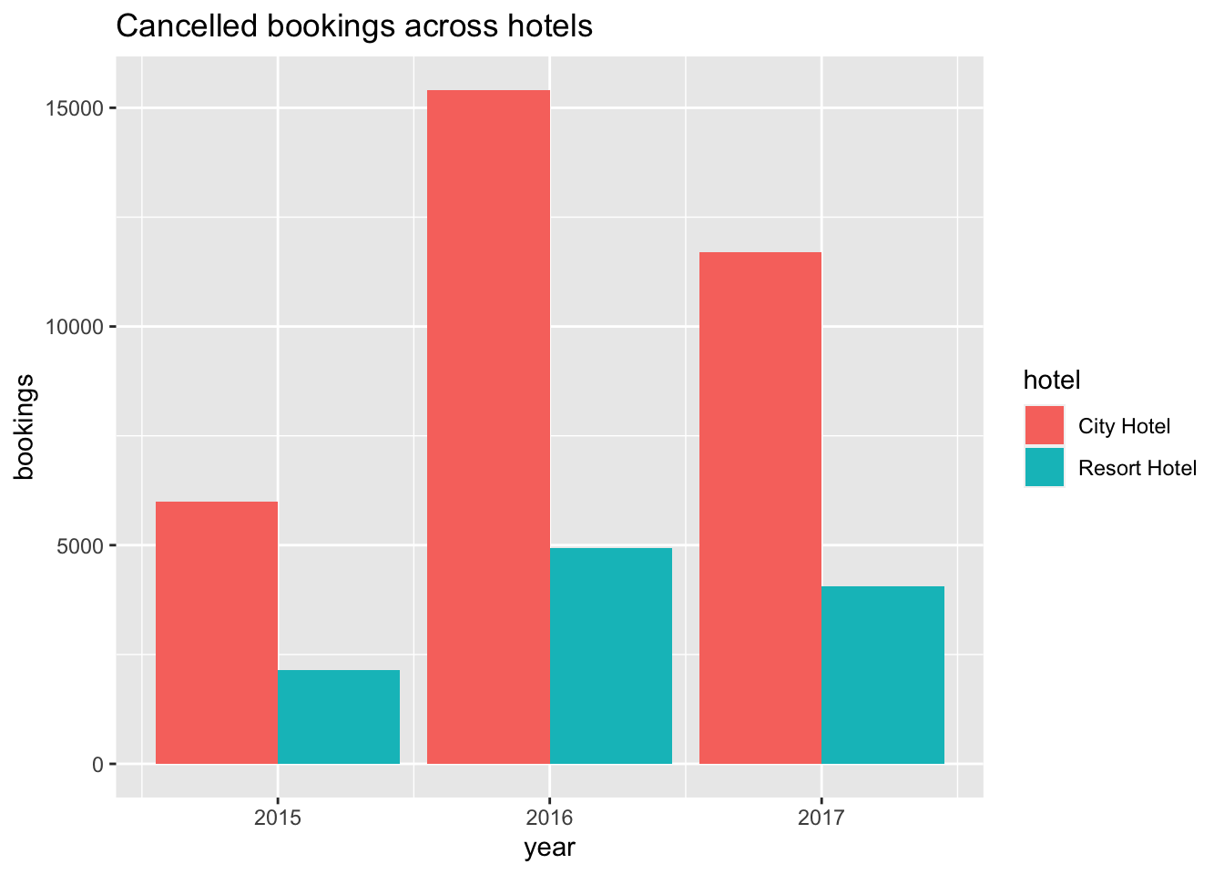
ggplot(data = cancelled_bookings_by_year, aes(x= arrival_date_year, y=no_bookings)) +
  geom_bar(stat = "identity", mapping = aes(fill = hotel), position = "dodge") +
  ggtitle("Cancelled bookings across hotels") +
  ylab("bookings") +
  xlab("year")

Code

not_cancelled_bookings_by_year <- hotel_booking_by_year %>% 
  filter(is_canceled == 0) %>%
  select(hotel, arrival_date_year, no_bookings)

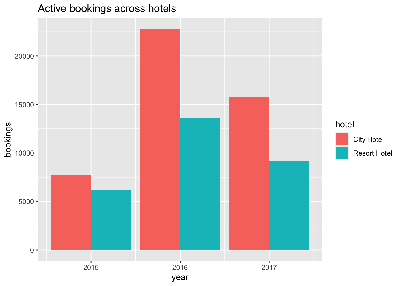
ggplot(data = not_cancelled_bookings_by_year, aes(x= arrival_date_year, y=no_bookings)) +
  geom_bar(stat = "identity", mapping = aes(fill = hotel), position = "dodge") +
  ggtitle("Active bookings across hotels") +
  ylab("bookings") +
  xlab("year")

Code

# Total number of bookings that are not cancelled per hotel
(actual_hotel_booking <- hotel_booking_by_year %>%
  filter(is_canceled == 0) %>%
  group_by(hotel) %>%
  summarise(no_bookings = sum(no_bookings)))

# A tibble: 2 × 2
  hotel        no_bookings
  <chr>              <int>
1 City Hotel         46228
2 Resort Hotel       28938

Code

# Mean, median and standard deviation of night stays
# during the week and weekends per hotel
(stay_pattern <- booking_data %>% 
  group_by(hotel) %>%
  summarise(mean_stay_week_nights = mean(stays_in_week_nights),
            median_stay_week_nights = median(stays_in_week_nights),
            sd_stay_week_nights = sd(stays_in_week_nights),
            mean_stay_weekend_nights = mean(stays_in_weekend_nights),
            median_stay_weekend_nights = median(stays_in_weekend_nights),
            sd_stay_weekend_nights = sd(stays_in_weekend_nights)))

# A tibble: 2 × 7
  hotel        mean_stay_week_nights median_stay_week_nights sd_stay_week_nights
  <chr>                        <dbl>                   <dbl>               <dbl>
1 City Hotel                    2.18                       2                1.46
2 Resort Hotel                  3.13                       3                2.46
# ℹ 3 more variables: mean_stay_weekend_nights <dbl>,
#   median_stay_weekend_nights <dbl>, sd_stay_weekend_nights <dbl>

Code

# Number of repeated guests who didn't cancel per hotel.
(repeated_guests <- booking_data %>%
  filter(is_repeated_guest == 1, is_canceled == 0) %>%
  group_by(hotel) %>%
  summarise(count = n()))

# A tibble: 2 × 2
  hotel        count
  <chr>        <int>
1 City Hotel    1591
2 Resort Hotel  1667

Explain and Interpret

Be sure to explain why you choose a specific group. Comment on the interpretation of any interesting differences between groups that you uncover. This section can be integrated with the exploratory data analysis, just be sure it is included.

Compared the number of booking across hotels on a yearly basis and tried to observe the retention rate among customers.We can see that in the period of 3 years, City Hotel has 46228 bookings that aren’t cancelled whereas Resort Hotel has 28938. Out of these, 3.4416371% and 5.7605916% are repeated bookings for City Hotel and Resort Hotel respectively. Although the number of bookings for City Hotel were higher, Resort Hotel has a better customer retention rate compared to City Hotel.