Code
library(tidyverse)
library(ggplot2)

knitr::opts_chunk$set(echo = TRUE, warning=FALSE, message=FALSE)library(tidyverse)
library(ggplot2)
knitr::opts_chunk$set(echo = TRUE, warning=FALSE, message=FALSE)Today’s challenge is to:
R Graph Gallery is a good starting point for thinking about what information is conveyed in standard graph types, and includes example R code.
(be sure to only include the category tags for the data you use!)
Read in one (or more) of the following datasets, using the correct R package and command.
stay_data <- read_csv("_data/AB_NYC_2019.csv")
head(stay_data)
# A tibble: 6 × 16
id name host_id host_name neighbourhood_group neighbourhood latitude
<dbl> <chr> <dbl> <chr> <chr> <chr> <dbl>
1 2539 Clean & qu… 2787 John Brooklyn Kensington 40.6
2 2595 Skylit Mid… 2845 Jennifer Manhattan Midtown 40.8
3 3647 THE VILLAG… 4632 Elisabeth Manhattan Harlem 40.8
4 3831 Cozy Entir… 4869 LisaRoxa… Brooklyn Clinton Hill 40.7
5 5022 Entire Apt… 7192 Laura Manhattan East Harlem 40.8
6 5099 Large Cozy… 7322 Chris Manhattan Murray Hill 40.7
# ℹ 9 more variables: longitude <dbl>, room_type <chr>, price <dbl>,
# minimum_nights <dbl>, number_of_reviews <dbl>, last_review <date>,
# reviews_per_month <dbl>, calculated_host_listings_count <dbl>,
# availability_365 <dbl>area_wise_stays <- stay_data %>%
group_by(neighbourhood_group, room_type) %>%
summarise(count = n())The AB_NYC_2019 provides information on Airbnb stays in New York in 2019. There are details about 48895 stays. They are distributed across Bronx, Brooklyn, Manhattan, Queens, Staten Island neighbourhoods. The below table shows the number of stay options across New York neighbourhood.
area_wise_stays# A tibble: 15 × 3
# Groups: neighbourhood_group [5]
neighbourhood_group room_type count
<chr> <chr> <int>
1 Bronx Entire home/apt 379
2 Bronx Private room 652
3 Bronx Shared room 60
4 Brooklyn Entire home/apt 9559
5 Brooklyn Private room 10132
6 Brooklyn Shared room 413
7 Manhattan Entire home/apt 13199
8 Manhattan Private room 7982
9 Manhattan Shared room 480
10 Queens Entire home/apt 2096
11 Queens Private room 3372
12 Queens Shared room 198
13 Staten Island Entire home/apt 176
14 Staten Island Private room 188
15 Staten Island Shared room 9Each stay option has information about id, name, host_id, host_name, neighbourhood_group, neighbourhood, latitude, longitude, room_type, price, minimum_nights, number_of_reviews, last_review, reviews_per_month, calculated_host_listings_count, availability_365.
Is your data already tidy, or is there work to be done? Be sure to anticipate your end result to provide a sanity check, and document your work here.
Variables like id and host_id are int but they are actually categorical. So, they have to be converted to factor. We can drop one of the columns out of “host_id” and “name” for exploratory analysis as they only act as primary keys. “last_review” column has to be converted to date format to represent the true data format. All character columns like neighbourhood_group, neighbourhood, etc have to be converted to factor to get better insights on using summary. After this step, summary will give value counts for categorical variables and there will be 15 columns.
stay_data <- stay_data %>%
  select(-name) %>%
  mutate_if(is.character, as.factor) %>%
  mutate(id = as.factor(id),
         host_id = as.factor(host_id),
         last_review = as.Date(last_review, format = "%Y-%m-%d"))

summary(stay_data)
id host_id host_name neighbourhood_group
2539 : 1 219517861: 327 Michael : 417 Bronx : 1091
2595 : 1 107434423: 232 David : 403 Brooklyn :20104
3647 : 1 30283594 : 121 Sonder (NYC): 327 Manhattan :21661
3831 : 1 137358866: 103 John : 294 Queens : 5666
5022 : 1 12243051 : 96 Alex : 279 Staten Island: 373
5099 : 1 16098958 : 96 (Other) :47154
(Other):48889 (Other) :47920 NA's : 21
neighbourhood latitude longitude
Williamsburg : 3920 Min. :40.50 Min. :-74.24
Bedford-Stuyvesant: 3714 1st Qu.:40.69 1st Qu.:-73.98
Harlem : 2658 Median :40.72 Median :-73.96
Bushwick : 2465 Mean :40.73 Mean :-73.95
Upper West Side : 1971 3rd Qu.:40.76 3rd Qu.:-73.94
Hell's Kitchen : 1958 Max. :40.91 Max. :-73.71
(Other) :32209
room_type price minimum_nights number_of_reviews
Entire home/apt:25409 Min. : 0.0 Min. : 1.00 Min. : 0.00
Private room :22326 1st Qu.: 69.0 1st Qu.: 1.00 1st Qu.: 1.00
Shared room : 1160 Median : 106.0 Median : 3.00 Median : 5.00
Mean : 152.7 Mean : 7.03 Mean : 23.27
3rd Qu.: 175.0 3rd Qu.: 5.00 3rd Qu.: 24.00
Max. :10000.0 Max. :1250.00 Max. :629.00
last_review reviews_per_month calculated_host_listings_count
Min. :2011-03-28 Min. : 0.010 Min. : 1.000
1st Qu.:2018-07-08 1st Qu.: 0.190 1st Qu.: 1.000
Median :2019-05-19 Median : 0.720 Median : 1.000
Mean :2018-10-04 Mean : 1.373 Mean : 7.144
3rd Qu.:2019-06-23 3rd Qu.: 2.020 3rd Qu.: 2.000
Max. :2019-07-08 Max. :58.500 Max. :327.000
NA's :10052 NA's :10052
availability_365
Min. : 0.0
1st Qu.: 0.0
Median : 45.0
Mean :112.8
3rd Qu.:227.0
Max. :365.0
Cleaned data has 15 columns. Summary shows value counts of categorical variables. The class of “last_review” is Date.
Are there any variables that require mutation to be usable in your analysis stream? For example, do you need to calculate new values in order to graph them? Can string values be represented numerically? Do you need to turn any variables into factors and reorder for ease of graphics and visualization?
Adding percent column to “area_wise_stays” tibble that has been created above by grouping original data based on “neighbourhood_group” and “room_type”.
(percent_rooms_in_area <- area_wise_stays %>%
  group_by(neighbourhood_group) %>%
  summarise(count = sum(count)) %>%
  mutate(percent = count * 100 / sum(count),
         id = LETTERS[row_number()]))
# A tibble: 5 × 4
neighbourhood_group count percent id
<chr> <int> <dbl> <chr>
1 Bronx 1091 2.23 A
2 Brooklyn 20104 41.1 B
3 Manhattan 21661 44.3 C
4 Queens 5666 11.6 D
5 Staten Island 373 0.763 E We have the percent distribution of rooms across New York as shown above and each row is tagged with a id.
# pie chart of above room distribution data
ggplot(percent_rooms_in_area,
       aes(x = "", y = percent,
           fill = paste(id,' - ',neighbourhood_group,'(',round(percent,2),'%)'))) +
  geom_bar(width = 10, stat = "identity", color = "black") +
  geom_text(aes(x = 2.5, label = id),
            position = position_stack(vjust=0.5),
            color = "black") +
  coord_polar("y", start = 0) +
  theme_void() +
  labs(title = "Stays in New York area",
       fill = "Area")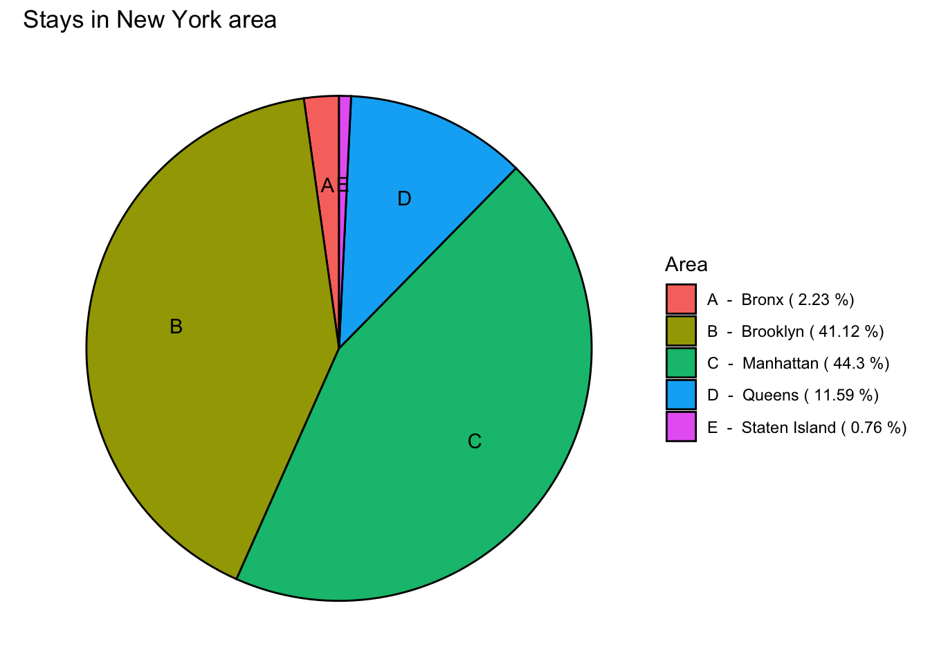
# box plot for availability in 365
ggplot(stay_data, mapping = aes(y = availability_365, fill = "orange")) +
  geom_boxplot() +
  theme(axis.title.y = element_blank(),
        axis.text.y = element_blank(),
        axis.ticks.y = element_blank(),
        legend.position = "none") +
  coord_flip() +
  labs(y = "Availability (Number of days in year)")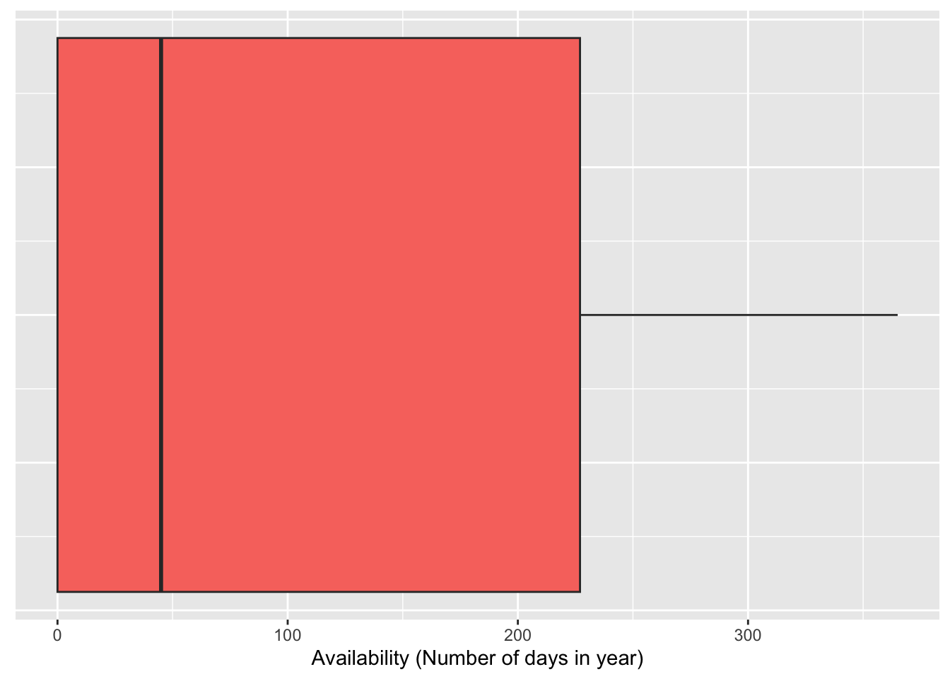
Pie chart has been chosen to show room distribution because “neighbourhood_group” is categorical variable. Box plot has been chosen to show availability of stays in New York as it is a quantitative variable and we can get some good statistical idea as well.
#Bar graph for room types in New York neighbourhood
ggplot(data = area_wise_stays, aes(x= room_type, y=count)) +
  geom_bar(stat = "identity",
           mapping = aes(fill = neighbourhood_group),
           position = "dodge") +
  labs(title ="Room types in New York neighbourhood",
       y = "Number of rooms",
       x = "Room Type",
       fill = "Area")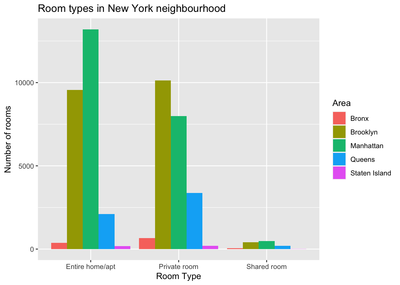
#Plot price distribution for each room type
ggplot(stay_data, aes(x = price, fill = room_type)) +
  geom_density(adjust =250, alpha = 0.5) +
  theme_linedraw() +
  facet_wrap(~room_type) +
  theme(legend.position = "none") +
  labs(title = "Price density for various room types in New York",
       x = "Price ($)")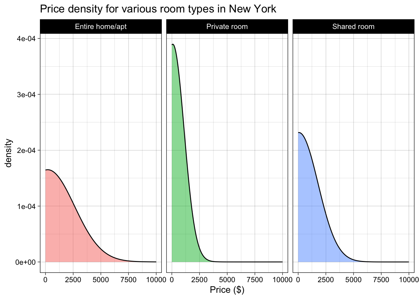
Bar plot has been chosen to show the number of rooms based on their types across New York area as the variable is categorical. Likewise, density plot has been chosen for price because it is a continuous variable. We can see that the standard deviation in prices is higher for entire home/shared room compared to private room throughout New York.