library(tidyverse)
library(ggplot2)
library(ggrepel)
knitr::opts_chunk$set(echo = TRUE, warning=FALSE, message=FALSE)
Challenge 8
Joining Data
Challenge Overview
Today’s challenge is to:
- read in multiple data sets, and describe the data set using both words and any supporting information (e.g., tables, etc)
- tidy data (as needed, including sanity checks)
- mutate variables as needed (including sanity checks)
- join two or more data sets and analyze some aspect of the joined data
(be sure to only include the category tags for the data you use!)
Read in data
- snl ⭐⭐⭐⭐⭐
There are three dataset about snl, which are actors, casts and seasons. I will join them.
actors <- read.csv("_data/snl_actors.csv")
casts <- read.csv("_data/snl_casts.csv")
seasons <- read.csv("_data/snl_seasons.csv")

actorscastsseasonsBriefly describe the data
in actors dataset, there are 4 columns. aid = actor id url = uniform resource locator type = the type of actors gender = actors’ gender
incasts dataset, there are 8 columns. sid = season id featured = whether the actor is featured player first_epid = the time of first episode of the actor last_epid = the time of last episode of the actor update_anchor = whether the actor is update anchor n_episodes = the number of episode of the actor season_fraction = the fraction of the total season
inseasons first_epid = the time of first episode last_epid = the time of last episode n_episodes = the number of episode ## Tidy Data (as needed) I rename the columns’ name at first which makes them clearer to see.
actors <- actors %>% rename(
  actor_id = aid,
  uniform_resource_locator = url
)

casts <- casts %>% rename(
  actor_id = aid,
  season_id = sid,
  actor_first_epid  = first_epid,
  actor_last_epid  = last_epid,
  actor_n_episodes = n_episodes
)

seasons <- seasons %>% rename(
  season_id = sid)
actors <- actors %>% rename(role_type = type)
actorscastsseasonscasts <- casts %>% fill(actor_first_epid, .direction = "down")
casts <- casts %>% mutate(actor_first_epid = date(actor_first_epid))
castsAre there any variables that require mutation to be usable in your analysis stream? For example, do you need to calculate new values in order to graph them? Can string values be represented numerically? Do you need to turn any variables into factors and reorder for ease of graphics and visualization?
Document your work here. ## Join Data
join <- actors %>% left_join(casts, by = "actor_id")
join <- join %>% left_join(seasons, by = "season_id")
join
join <- join %>% select(-year) %>%
mutate(season_id = as.character(season_id),
featured = as.logical(featured),
update_anchor = as.logical(update_anchor))
join <- join %>% mutate(first_epid = date(first_epid),
last_epid = date(last_epid))
joinAnalysis
join %>% ggplot(aes(x=gender, y=actor_n_episodes, fill = gender)) +
  geom_bar(position="stack", stat="identity") +
  labs(title = "The Relationship of Gender and Total Episodes of Actors",
       x = "Gender",
       y = "Total Episodes") +
  theme(axis.title.y = element_text(angle=0)) +
theme_minimal() 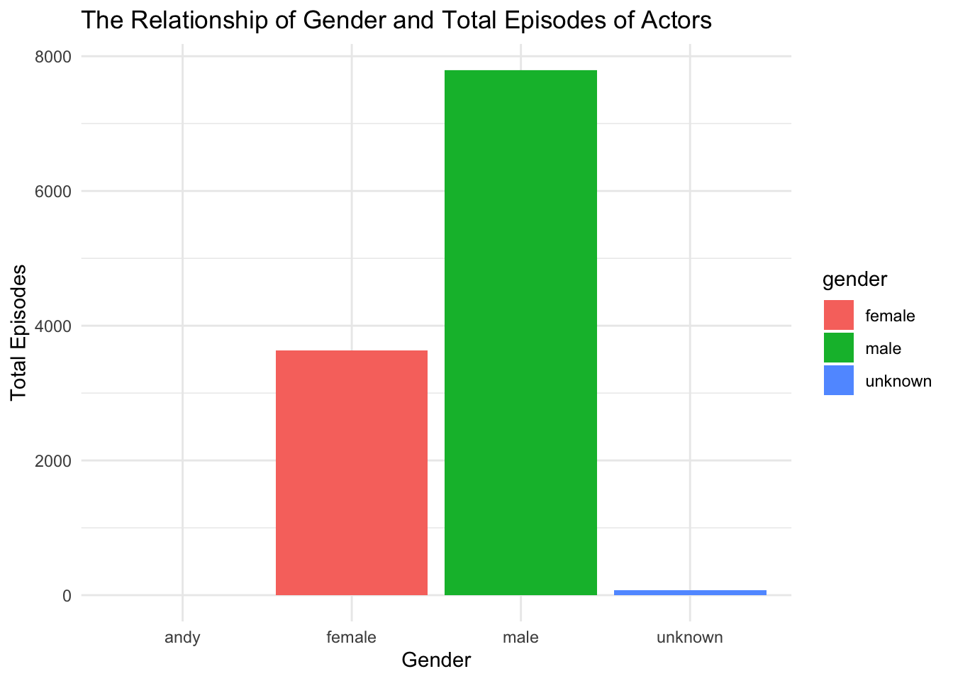
Here’s an unclear gender called “andy”. From below tibble, we can see there are just 21 “andy” gender which are not so many, so we can classify them into unknown
join %>% group_by(gender) %>% summarise(n=n())join <- join %>% mutate( gender = case_when(
gender == "andy" ~ "unknown",
gender == "male" ~ "male",
gender == "female" ~ "female",
gender == "unknown" ~ "unknown"
))
joinjoin %>% ggplot(aes(x=gender, y=actor_n_episodes, fill = gender)) +
geom_bar(position="stack", stat="identity") +
labs(title = "The Relationship of Gender and Total Episodes of Actors",
x = "Gender",
y = "Total Episodes") +
theme(axis.title.y = element_text(angle=0)) +
theme_minimal() 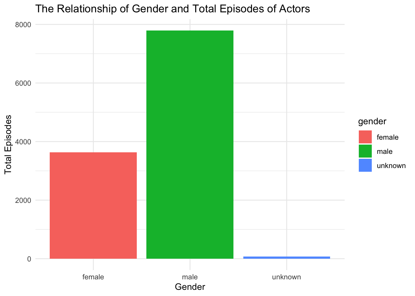
We can see here’s the new graph of the relationship between gender and total episodes of actors. It’s obvious that male actors have much more episodes than female actors have.
join %>% group_by(update_anchor,gender) %>% summarize(avg_actor_seasons = mean(actor_n_episodes)) %>% filter(!is.na(avg_actor_seasons)) %>%
  ggplot(aes(x=update_anchor, y = avg_actor_seasons, fill = gender)) +
  geom_bar( stat="identity") +
theme_minimal() 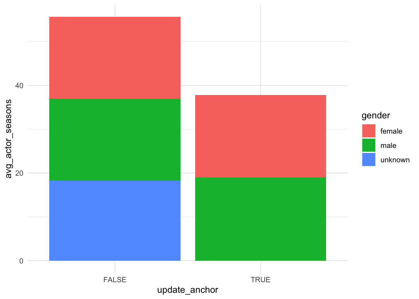
join %>% group_by(update_anchor,gender) %>% summarize(avg_actor_seasons = mean(actor_n_episodes)) %>% filter(!is.na(avg_actor_seasons)) %>%
  ggplot(aes(x=gender, y = avg_actor_seasons, fill = update_anchor)) +
  geom_bar( stat="identity") +
  facet_wrap(~update_anchor, drop = TRUE) +
  theme_minimal() +
  geom_text_repel(aes(label = avg_actor_seasons))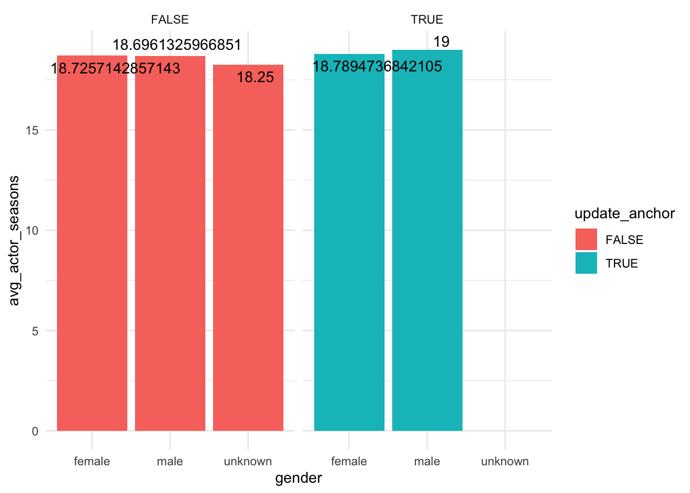
From the first graph, we can see the the number of average seasons of actors who are not update anchor is more than who are update anchor. And we can see the proportions of every gender are almost equal.
From the second graph, we can confirm that no matter the actors are update anchor, the number of average seasons of all genders is almost the same.