Challenge 8 Post: Joining FAOSTAT Datasets

challenge_8

faostat

Joining Data

Author

Hunter Major

Published

June 27, 2023

library(tidyverse)
library(ggplot2)
library(readxl)
library(readr)
library(lubridate)
library(dplyr)
library(tidyr)
knitr::opts_chunk$set(echo = TRUE, warning=FALSE, message=FALSE)

Challenge Overview

Today’s challenge is to:

read in multiple data sets, and describe the data set using both words and any supporting information (e.g., tables, etc)
tidy data (as needed, including sanity checks)
mutate variables as needed (including sanity checks)
join two or more data sets and analyze some aspect of the joined data

(be sure to only include the category tags for the data you use!)

Read in data

Read in one (or more) of the following datasets, using the correct R package and command.

Today, I’ll be reading in faostat ⭐⭐

cattledairy <-read_csv("_data/FAOSTAT_cattle_dairy.csv")
cattledairy

countrygroups <- read_csv ("_data/FAOSTAT_country_groups.csv")
countrygroups

dim(cattledairy)

[1] 36449    14

head(cattledairy)

str(cattledairy)

spc_tbl_ [36,449 × 14] (S3: spec_tbl_df/tbl_df/tbl/data.frame)
 $ Domain Code     : chr [1:36449] "QL" "QL" "QL" "QL" ...
 $ Domain          : chr [1:36449] "Livestock Primary" "Livestock Primary" "Livestock Primary" "Livestock Primary" ...
 $ Area Code       : num [1:36449] 2 2 2 2 2 2 2 2 2 2 ...
 $ Area            : chr [1:36449] "Afghanistan" "Afghanistan" "Afghanistan" "Afghanistan" ...
 $ Element Code    : num [1:36449] 5318 5420 5510 5318 5420 ...
 $ Element         : chr [1:36449] "Milk Animals" "Yield" "Production" "Milk Animals" ...
 $ Item Code       : num [1:36449] 882 882 882 882 882 882 882 882 882 882 ...
 $ Item            : chr [1:36449] "Milk, whole fresh cow" "Milk, whole fresh cow" "Milk, whole fresh cow" "Milk, whole fresh cow" ...
 $ Year Code       : num [1:36449] 1961 1961 1961 1962 1962 ...
 $ Year            : num [1:36449] 1961 1961 1961 1962 1962 ...
 $ Unit            : chr [1:36449] "Head" "hg/An" "tonnes" "Head" ...
 $ Value           : num [1:36449] 700000 5000 350000 700000 5000 ...
 $ Flag            : chr [1:36449] "F" "Fc" "F" "F" ...
 $ Flag Description: chr [1:36449] "FAO estimate" "Calculated data" "FAO estimate" "FAO estimate" ...
 - attr(*, "spec")=
  .. cols(
  ..   `Domain Code` = col_character(),
  ..   Domain = col_character(),
  ..   `Area Code` = col_double(),
  ..   Area = col_character(),
  ..   `Element Code` = col_double(),
  ..   Element = col_character(),
  ..   `Item Code` = col_double(),
  ..   Item = col_character(),
  ..   `Year Code` = col_double(),
  ..   Year = col_double(),
  ..   Unit = col_character(),
  ..   Value = col_double(),
  ..   Flag = col_character(),
  ..   `Flag Description` = col_character()
  .. )
 - attr(*, "problems")=<externalptr>

dim(countrygroups)

[1] 1943    7

head(countrygroups)

str(countrygroups)

spc_tbl_ [1,943 × 7] (S3: spec_tbl_df/tbl_df/tbl/data.frame)
 $ Country Group Code: num [1:1943] 5100 5100 5100 5100 5100 5100 5100 5100 5100 5100 ...
 $ Country Group     : chr [1:1943] "Africa" "Africa" "Africa" "Africa" ...
 $ Country Code      : num [1:1943] 4 7 53 20 233 29 35 32 37 39 ...
 $ Country           : chr [1:1943] "Algeria" "Angola" "Benin" "Botswana" ...
 $ M49 Code          : chr [1:1943] "012" "024" "204" "072" ...
 $ ISO2 Code         : chr [1:1943] "DZ" "AO" "BJ" "BW" ...
 $ ISO3 Code         : chr [1:1943] "DZA" "AGO" "BEN" "BWA" ...
 - attr(*, "spec")=
  .. cols(
  ..   `Country Group Code` = col_double(),
  ..   `Country Group` = col_character(),
  ..   `Country Code` = col_double(),
  ..   Country = col_character(),
  ..   `M49 Code` = col_character(),
  ..   `ISO2 Code` = col_character(),
  ..   `ISO3 Code` = col_character()
  .. )
 - attr(*, "problems")=<externalptr>

Briefly describe the data

These FAOSTAT datasets are likely sourced from the United Nation’s Food and Agriculture Association (FAO). They provide information about the livestock and agriculture of various nations.

The FAOSTAT_cattle_dairy dataset contains data on dairy cattle and has 36,449 observations and 14 columns/variables. It has the following variables: Domain Code, Domain, Area Code, Area, Element Code, Element, Item Code, Item, Year Code, Year, Unit, Value, Flag, and Flag Description.
The FAOSTAT_country_groups dataset contains data on country groups and various countries. It has 1,943 observations and 7 columns/variables. The variables in this dataset are as follows: Country Group Code, Country Group, Country Code, Country, M49 Code, ISO2 Code, and ISO3 Code.

Tidy Data (as needed)

Is your data already tidy, or is there work to be done? Be sure to anticipate your end result to provide a sanity check, and document your work here.

The data is already tidy.

Mutating Variables

Are there any variables that require mutation to be usable in your analysis stream? For example, do you need to calculate new values in order to graph them? Can string values be represented numerically? Do you need to turn any variables into factors and reorder for ease of graphics and visualization?

There seems to be a good opportunity to join the Country variable of FAOSTAT_country_groups with the Area variable of FAOSTAT_cattle_dairy. Within the FAOSTAT_country_groups dataset, the only variable I will be joining with the FAOSTAT_cattle_dairy dataset is the Country variable, so before doing so, I will remove the other variables from the FAOSTAT_country_groups dataset. I don’t think this is the best practice in real-world data cleaning as it deletes a lot of data, but for the purposes of this joining exercise and to pair down the amount of information I’ll have in the joined dataset (to something that’s more concise, relevant, and useful for this challenge); this seems convenient to me.

# removing all variables except Country from FAOSTAT_country_groups
countrygroups2 <- countrygroups %>% select(-c(`Country Group Code`, `Country Group`, `Country Code`, `M49 Code`, `ISO2 Code`, `ISO3 Code`))
countrygroups2

# check for new dimensions
dim(countrygroups2)

[1] 1943    1

Now there’s one variable, Country, and 1,943 rows in the countrygroups2 dataset.

I also feel like I can pair down on the variables in the FAOSTAT_cattle_dairy dataset, so I will be removing the following variables for convenience: - Domain - Domain Code - Area Code - Element Code - Item - Item Code - Year Code - Flag - Flag Description

# removing unnecessary variables from FAOSTAT_cattle_dairy
cattledairy2 <- cattledairy %>% select(-c(`Domain`, `Item`, `Domain Code`, `Area Code`, `Element Code`, `Item Code`, `Year Code`, `Flag`, `Flag Description`))
cattledairy2

#check for new dimensions
dim(cattledairy2)

[1] 36449     5

Now, there’s 5 variables and 36,449 observations in cattledairy2.

Join Data

Be sure to include a sanity check, and double-check that case count is correct!

#joining Country to Area from countrygroups2 to cattledairy2
joincattlecountry <- inner_join(cattledairy2, countrygroups2,
                                 by = c("Area" = "Country"))
joincattlecountry

#getting rid of repeat rows
joincattlecountry2 <- unique(joincattlecountry)
joincattlecountry2

#pair down to years 2000-2004
joincattlecountry3 <- joincattlecountry2[joincattlecountry2$Year >= "2000" & joincattlecountry2$Year <= "2004",]
joincattlecountry3

I got rid of repeating rows and further paired the dataset down just to range from years 2000-2004.

Data Visualization

# Scatterplot of Value over Time Sorted by Element
ggplot(joincattlecountry3, aes(x= Year, y= Value, fill= Element))+
  geom_point(shape= 21, color="black", size= 2)+
  labs(title= "A Scatterplot of Dairy Cattle Value sorted by Element", subtitle = "2000-2004", x= "Year", y= "Value", fill= "Element")+
  theme(axis.text.x = element_text(angle = 30, size = 2))+
  facet_grid()+
  theme_minimal()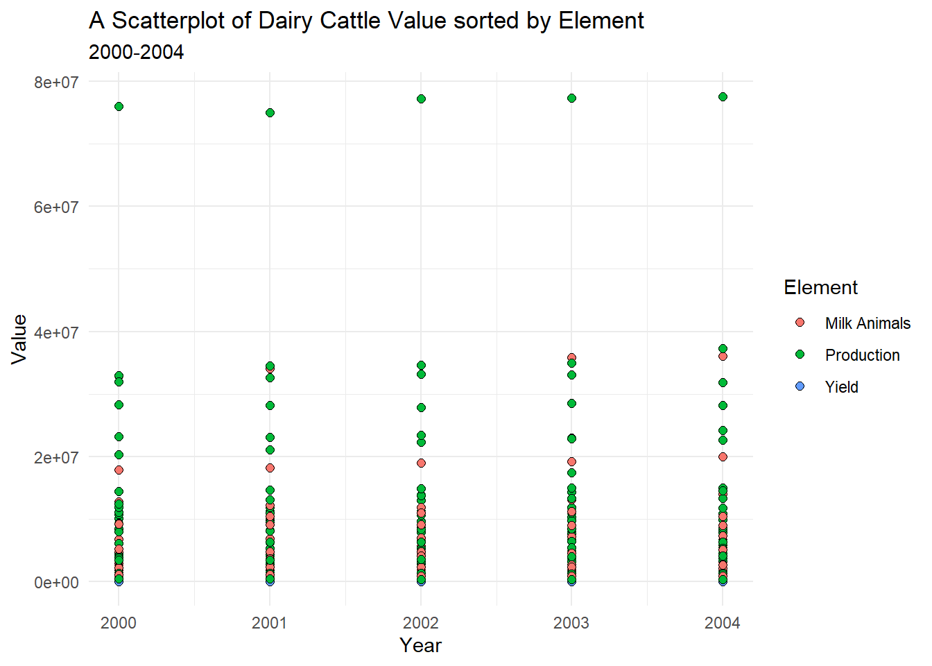

Using Pivot-Wider to get country specific-data

#using pivot wider to get country specific data
joincattlecountry4 <- joincattlecountry3 %>% pivot_wider(names_from = Element, values_from = Value)
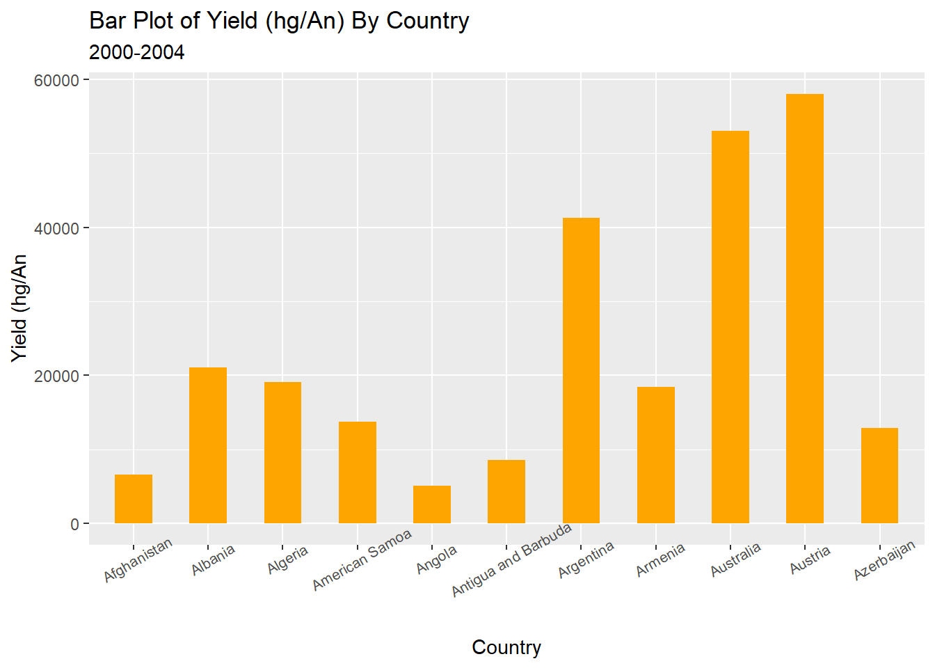
joincattlecountry4

#pair down to Areas starting with letter "A": Afghanistan-Azerbaijan
joincattlecountry5 <- joincattlecountry4[joincattlecountry4$Area >= "Afghanistan" & joincattlecountry4$Area <= "Azerbaijan",]
joincattlecountry5

#Bar Plot of Yield Value by Country
ggplot(joincattlecountry5, aes(x= Area, y= Yield))+
         geom_bar(width= .5, stat="identity", fill="orange", position= position_dodge(width = .8))+
         facet_grid()+
         theme(axis.text.x = element_text(angle = 30, size = 8))+
         labs(title = "Bar Plot of Yield (hg/An) By Country", subtitle= "2000-2004", x= "Country", y= "Yield (hg/An")