Challenge 8 Solutions

library(tidyverse)
library(readxl)
library(here)

knitr::opts_chunk$set(echo = TRUE, warning=FALSE,
                      message=FALSE)

Challenge Overview

1. read in multiple data sets, and describe the data set using both words and any supporting information (e.g., tables, etc)
2. tidy data (as needed, including sanity checks)
3. mutate variables as needed (including sanity checks)
4. join two or more data sets and analyze some aspect of the joined data

(be sure to only include the category tags for the data you use!)

Read in data

Read in one (or more) of the following datasets, using the correct R package and command.

• military marriages ⭐⭐
• faostat ⭐⭐
• railroads ⭐⭐⭐
• fed_rate ⭐⭐⭐
• debt ⭐⭐⭐
• us_hh ⭐⭐⭐⭐
• snl ⭐⭐⭐⭐⭐

:::{.panel-tabset}

Military Marriages

The excel workbook “ActiveDuty_MaritalStatus.xls” contains tabulations of total number of active duty military members classified by marital and family status, for each of the branches of military as well as the military overall. The sheet is a typical government table, so lets figure out what information is actually available! After that, we will clean a single sheet from the workbook, and use that effort to create a generic function that can be used to iterate through all sheets in the workbook to read them and then join them together into a single dataset.

Find Information available

Lets first look at an example sheet from the workbook.

Total DOD Active Duty Marital Sheet

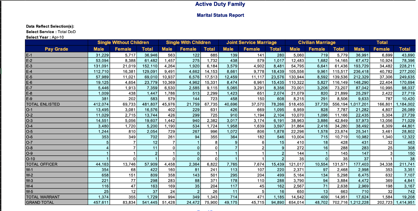
We can see a few things from this example sheet. First, we will need to skip 8 or 9 rows - the data first appears in row 10. Second, the tabular cells represent count values that capture the number of employees falling into subcategories created by 6 distinct grouping values: 1) Pay Grade Type: Enlisted/Officer/Warrant Officer 2) Pay Grade Level: 1-10 (fewer for non-Enlisted) 3) Marital status: Married/Single 4) Parent: Kids/noKids (Single only) 5) Spouse affiliation: Civilian/Military (Married only) 6) Gender: Male/Female

Our goal is to recover cases that have these 6 (or really 5, if we collapse parent and spouse variables as we don’t have complete information) grouping variables to identify the case and the single value (count of active duty employees who fall into each of the resulting subcategories.)

Looking back at the original excel sheet, we can see that we will need to not just skip the top rows, we will also need to delete several columns, and also rename variables in order to make it easy to separate out the three pieces of information contained in the column names. First, I create a vector with column names (to make it easier to reuse later when I pivot to tidy data) then I read in the data and inspect it to see if the columns worked as intended.

marital_cols <-c("d", "payGrade_payLevel",
            "single_nokids_male", "single_nokids_female", "d",
            "single_kids_male", "single_kids_female", "d",
            "married_military_male", "married_military_female", "d",
            "married_civilian_male", "married_civilian_female", "d",
            rep("d", 3))

read_excel(here("posts","_data","ActiveDuty_MaritalStatus.xls"), 
           skip=8,
           col_names = marital_cols)

I can see that the variable names worked well, so this time I will read in the data and omit the original header row, and also filter out the various “TOTAL” rows that we don’t need to keep.

Read in single sheet

military<-read_excel(here("posts","_data","ActiveDuty_MaritalStatus.xls"), 
           skip=9,
           col_names = marital_cols
           )%>%
  select(!starts_with("d"))%>%
  filter(str_detect(payGrade_payLevel, "TOTAL", negate=TRUE))

military

It looks like this worked well! Now we just need to pivot_longer with 3 columns, then separate out the information in the payGrade_payLevel variable and do a quick mutate to make paygrade easier to remember.

military_long <-military %>%
  pivot_longer(cols = -1,
               names_to = c("Marital", "Other", "Gender"),
               names_sep = "_",
               values_to = "count")%>%
  separate(payGrade_payLevel, 
           into = c("payGrade", "payLevel"),
           sep="-")%>%
  mutate(payGrade = case_when(
    payGrade == "E" ~ "Enlisted",
    payGrade == "O" ~ "Officer",
    payGrade == "W" ~ "Warrant Officer"
  ))

military_long

This all looks like it works well. So now we will go on to creating a function with the steps, then applying it to multiple sheets.

Create data reading function

We will call our new function read_military, and we will basically use the exact same commands as above. The big difference is that we will have a placeholder name (or argument) for the data sheet that will be passed to the new function.

Another difference is that when using read_excel() on a workbook with multiple sheets, we need to specify the sheetname of the sheet we wish to read in (we can also specify the sheet name). I then include the mutate() command to create a new column called branch, which comes from our sheet name.

Everything else will be pretty identical to reading a single sheet - select(!starts_with("d")) removes all columns that start with "d". We also filter out the word “Total” from payGrade_payLevel. pivot_longer()

read_military<-function(sheet_name){
  dat <- read_excel(here("posts","_data","ActiveDuty_MaritalStatus.xls"), 
             sheet = sheet_name,
             skip=9,
             col_names = marital_cols
             )%>%
    mutate(branch=sheet_name) %>%
    select(!starts_with("d"))%>%
    filter(str_detect(payGrade_payLevel, "TOTAL", negate=TRUE))%>%
    pivot_longer(cols = contains(c("male", "female")),
                 names_to = c("Marital", "Other", "Gender"),
                 names_sep = "_",
                 values_to = "count")%>%
    separate(payGrade_payLevel, 
             into = c("payGrade", "payLevel"),
             sep="-")%>%
    mutate(payGrade = case_when(
      payGrade == "E" ~ "Enlisted",
      payGrade == "O" ~ "Officer",
      payGrade == "W" ~ "Warrant Officer"
    ))
  return(dat)
}

Purrr to join

We now have a function that is customized to read in the military active duty marital status sheets. We just need to use purrr - a package that is part of tidyverse but which may need to be installed and loaded on its own - to iterate through the list of sheets in the workbook.

military_sheets<-excel_sheets(here("posts","_data","ActiveDuty_MaritalStatus.xls") )

military_sheets

[1] "TotalDoD"    "AirForce"    "MarineCorps" "Navy"        "Army"       

Now we have a list of sheet names to map with the function. Typically, a purrr::map_() function creates a list of data frames with each element in the original vector fed to the function as a single list element, as depicted below.

We are going to use map_dfr() to join the four elements of the list into a single dataframe. map is the generic purrr function, and adding on the dfr means that we want to turn all of the list elements created by map into a single dataframe (df) that is joined by rows (r).

using map_dfr

There are functions in purrr that automatically convert the list created by map into the dataframe shape that you want, but you need to be careful that the objects being mapped have the correct column names (or rows, if you are using map_dfc() to avoid errors. Plain map is the safe option, but you then have to manually join the data.)

military_all <- map_dfr(
  excel_sheets(here("posts","_data","ActiveDuty_MaritalStatus.xls"))[-1],
  read_military)
military_all

FAOstat Regions

The FAOSTAT sheets are excerpts of the FAOSTAT database provided by the Food and Agriculture Association, an agency of the United Nations. There are two approaches we could use to joining these data. In this section, we are going to join livestock estimates from a single file to regional codes for the countries.

The file birds.csv that includes estimates of the stock of five different types of poultry (Chickens, Ducks, Geese and guinea fowls, Turkeys, and Pigeons/Others) in 248 areas for 58 years between 1961-2018. Because we know (from challenge 1) that several of those areas include aggregated data (e.g., ) we are going to remove the aggregations and replace the case level aggregations with the correct grouping variables from the file “FAOSTAT_country_groups.csv”, downloaded from Country Region definitions provided by the FAO. As a reminder, I am going to split the original birds data into country level and aggregated data, and then list the aggregated groups we found in Challenge 1.

birds_orig<-read_csv(here("posts","_data","birds.csv"))%>%
  select(-contains("Code"))

birds_agg<-birds_orig%>%
  filter(Flag=="A")

birds<-birds_orig%>%
  filter(Flag!="A")

unique(birds_agg$Area)

 [1] "World"                     "Africa"                   
 [3] "Eastern Africa"            "Middle Africa"            
 [5] "Northern Africa"           "Southern Africa"          
 [7] "Western Africa"            "Americas"                 
 [9] "Northern America"          "Central America"          
[11] "Caribbean"                 "South America"            
[13] "Asia"                      "Central Asia"             
[15] "Eastern Asia"              "Southern Asia"            
[17] "South-eastern Asia"        "Western Asia"             
[19] "Europe"                    "Eastern Europe"           
[21] "Northern Europe"           "Southern Europe"          
[23] "Western Europe"            "Oceania"                  
[25] "Australia and New Zealand" "Melanesia"                
[27] "Micronesia"                "Polynesia"                

With the FAO regional information, we can find out which countries are in which regions:

fao_regions_orig <-read_csv(here("posts","_data","FAOSTAT_country_groups.csv"))
fao_regions<-fao_regions_orig%>%
  select(`Country Group`, Country)%>%
  rename(country_group = `Country Group`)%>%
  distinct()

fao_regions%>%
  filter(country_group == "Polynesia")

Clearly, some of the groups might overlap. For example, one group is called World and clearly overlaps with all other groups. So, before we join, lets remove the World group and then inspect the country-region pairings to ensure there are no other overlaps.

temp<-fao_regions%>%
  group_by(country_group)%>%
  summarize(n=n())%>%
  arrange(desc(n))
half <-c(1:round(nrow(temp)/2))
knitr::kable(list(temp[half,],  
           matrix(numeric(), nrow=0, ncol=1),
           temp[-half,]), 
           caption = "Countries in Country Groups")%>%
  kableExtra::kable_styling(font_size=12)

Countries in Country Groups

country_group n World 277 Non-Annex I countries 161 Net Food Importing Developing Countries 81 Annex I countries 78 High-income economies 64 Africa 63 Europe 63 Americas 61 Small Island Developing States 58 Upper-middle-income economies 56 Low Income Food Deficit Countries 55 Asia 54 Sub-Saharan Africa 53 Latin America and the Caribbean 52 Least Developed Countries 51 Sub-Saharan Africa (including Sudan) 49 Lower-middle-income economies 46 Northern America and Europe 44 OECD 36 Oceania 35 Low income economies 34 Land Locked Developing Countries 32 Caribbean 30 European Union (27) 30 Western Asia and Northern Africa 24 Eastern Africa 23 Eastern Asia and South-eastern Asia 20 Southern Europe 20 Western Asia 20

country_group n Northern Europe 18 Oceania excluding Australia and New Zealand 18 Western Africa 18 South America 17 Central Asia and Southern Asia 14 North and Central America 14 Western Asia (exc. Armenia, Azerbaijan, Cyprus, Israel and Georgia) 13 Eastern Europe 12 Polynesia 12 South-eastern Asia 11 Western Europe 11 Micronesia 10 Eastern Asia 9 Middle Africa 9 Southern Asia 9 Caucasus and Central Asia 8 Central America 8 Northern Africa 8 Southern Asia (excluding India) 8 Australia and New Zealand 6 Eastern Asia (excluding Japan) 6 Northern Africa (excluding Sudan) 6 Northern America 6 Central Asia 5 Melanesia 5 Southern Africa 5 Eastern Asia (excluding China) 3 Eastern Asia (excluding Japan and China) 3 Antarctic Region 1

temp

Unfortunately, we can see that many regions must overlap - which is super annoying. We need to essentially extract the country-level or regional groupings - of which there seem to be up to 7 or 8 - potentially nested or perhaps not - country grouping categories - to fully disentangle the various aggregations contained in the original data. The demonstration below quickly identifies four major grouping categories to extract and confirms that there are approximately 277 countries (or less) in each grouping category. More detailed work could be used to nest sub-regions within regions (e.g., Eastern Europe would nest within Europe, and so on.)

fao_regions%>%
  summarise(n=n())/277

fao_regions%>%
  filter(str_detect(country_group, "[aA]nnex"))%>%
  group_by(country_group)%>%
  summarise(n=n())

fao_regions%>%
  filter(str_detect(country_group, "[aA]nnex"))%>%
  summarise(n=n())

fao_regions%>%
  filter(str_detect(country_group, "[iI]ncome"))%>%
  group_by(country_group)%>%
  summarise(n=n())

fao_regions%>%
  filter(str_detect(country_group, "[iI]ncome"))%>%
  summarise(n=n())

fao_regions%>%
  filter(str_detect(country_group, "[Dd]evelop|OECD"))%>%
  group_by(country_group)%>%
  summarise(n=n())

fao_regions%>%
  filter(str_detect(country_group, "[Dd]evelop|OECD"))%>%
  summarise(n=n())

major_regions<-c("Africa", "Asia", "Europe", "Americas", 
                 "Oceania", "Antarctic Region")

fao_regions%>%
  filter(country_group %in% major_regions)%>%
  summarise(n=n())

We now use the unite() command to create four new categorical variables corresponding to the four country groupings we have identified that contain most or all of the 277 countries included in the data.

fao_regions_wide<-fao_regions%>%
  filter(country_group!="World")%>%
  pivot_wider(names_from=country_group, values_from = 1)%>%
  unite("gp_annex", contains("Annex"), 
        sep="", na.rm=TRUE, remove=TRUE)%>%
  unite("gp_major_region", any_of(major_regions), 
        sep="", na.rm=TRUE, remove=TRUE)%>%
  unite("gp_income", contains("Income")|contains("income"),
        sep="", na.rm=TRUE, remove=TRUE)%>%
  unite("gp_develop", contains("Develop")|contains("OECD"),
        sep="", na.rm=TRUE, remove=TRUE)%>%
  select(Country, starts_with("gp")) %>%
  mutate(across(starts_with("gp"),~na_if(.x,"")))
fao_regions_wide

Join to livestock data

Now that we have countries and four regional breakdown indicators, we can join this data to our original livestock data by country name. I am going to do a left_join, as each case includes a country, and we want to match countries to join the four regional indicators. Because the Country variable is described as Area in the original birds data, we want to explicitly set the two key fields for the join.

We should end up with the same number of rows in the “birds” data as we started off with. An inner_join would also work in this case, would effectively omit from the left-hand side data any aggregated cases left in by mistake (it would only keep rows where “Area” matched one of the “Country” values.)

nrow(birds)

[1] 13716

birds <- left_join(birds, fao_regions_wide,
                   by = c("Area" = "Country"))

Now, you can summarize across countries grouped by income, development status, major region, or Annex/non-Annex.

FAOstat: Regions

The FAOSTAT sheets are excerpts of the FAOSTAT database provided by the Food and Agriculture Association, an agency of the United Nations. There are two approaches we could use to joining these data. In this section, we are going to join livestock estimates from multiple “faostat…” files.

We have already seen that the file birds.csv includes estimates of the stock of five different types of poultry (Chickens, Ducks, Geese and guinea fowls, Turkeys, and Pigeons/Others) in 248 areas for 58 years between 1961-2018. What about the other “FAOSTAT_*” files?

Lets read them into a single list, and see what we find. First, lets write a function to just read in the file and then print out the column names.

list.files()

There are base R functions that allow you to easily interact with the underlying system, just like you would at the command line or in the terminal. One of my favorites is list.files(), which does exactly what it says on the tin! The pattern matching used in the terminal may vary slightly depending on your operating system.

read_faostat<-function(fn){
  fao<-read_csv(str_c(here("posts","_data"), fn, sep="/"))%>%
    select(-contains("Code"))
  
  return(colnames(fao))
}

fao_files<-list.files(path=here("posts","_data"), pattern="FAOSTAT*")
fao_files[2]<-"birds.csv"

map(fao_files, read_faostat)

[[1]]
[1] "Domain"           "Area"             "Element"          "Item"            
[5] "Year"             "Unit"             "Value"            "Flag"            
[9] "Flag Description"

[[2]]
[1] "Domain"           "Area"             "Element"          "Item"            
[5] "Year"             "Unit"             "Value"            "Flag"            
[9] "Flag Description"

[[3]]
[1] "Domain"           "Area"             "Element"          "Item"            
[5] "Year"             "Unit"             "Value"            "Flag"            
[9] "Flag Description"

[[4]]
[1] "Domain"           "Area"             "Element"          "Item"            
[5] "Year"             "Unit"             "Value"            "Flag"            
[9] "Flag Description"

We can see from this that the column names are identical in the four datasets, which makes them easy to merge. Additionally, we suspect from the birds dataset that the Domain variable will uniquely identify the dataset, lets see if we are correct by modifying our read_faostat function.

read_faostat<-function(fn){
  fao<-read_csv(str_c(here("posts","_data"), fn, sep="/"))%>%
    select(-contains("Code"))
  
  return(list(Domain = unique(fao$Domain),
              Elements = unique(fao$Element),
              Items = unique(fao$Item),
              obs = nrow(fao)))
}

map(fao_files, read_faostat)

[[1]]
[[1]]$Domain
[1] "Livestock Primary"

[[1]]$Elements
[1] "Milk Animals" "Yield"        "Production"  

[[1]]$Items
[1] "Milk, whole fresh cow"

[[1]]$obs
[1] 36449


[[2]]
[[2]]$Domain
[1] "Live Animals"

[[2]]$Elements
[1] "Stocks"

[[2]]$Items
[1] "Chickens"               "Ducks"                  "Geese and guinea fowls"
[4] "Turkeys"                "Pigeons, other birds"  

[[2]]$obs
[1] 30977


[[3]]
[[3]]$Domain
[1] "Livestock Primary"

[[3]]$Elements
[1] "Laying"     "Yield"      "Production"

[[3]]$Items
[1] "Eggs, hen, in shell"

[[3]]$obs
[1] 38170


[[4]]
[[4]]$Domain
[1] "Live Animals"

[[4]]$Elements
[1] "Stocks"

[[4]]$Items
[1] "Asses"     "Camels"    "Cattle"    "Goats"     "Horses"    "Mules"    
[7] "Sheep"     "Buffaloes" "Pigs"     

[[4]]$obs
[1] 82116

What an easy way to learn a lot about the data quickly. Sure enough, we can now merge the data back together and have way too much information in the same R object :-) This time, we will modify the read_faostat function to only read in the data, and then use purrr::map_dfr() to join.

read_faostat<-function(fn){
  fao<-read_csv(str_c(here("posts","_data"), fn, sep="/"))%>%
    select(-contains("Code"))
  return(fao)
}

faostat<- map_dfr(fao_files, read_faostat)%>%
  inner_join(fao_regions_wide, 
             by=c("Area" = "Country"))

faostat

SNL

The Data

These data came to my attention courtesy of Jeremy Singer-Vine’s wonderful Data is Plural newsletter. These datasets, archived by Joel Navaroli and scraped by Hendrik Hilleckes and Colin Morris, contain data about the actors, cast, seasons, etc. from every season of Saturday Night Live from its inception through 2020.

We will be working with three data files: actors.csv, casts.csv, and seasons.csv.

Now let’s read in the data.

actors <- read_csv(here("posts","_data","snl_actors.csv"))
casts <- read_csv(here("posts","_data","snl_casts.csv"))
seasons <- read_csv(here("posts","_data","snl_seasons.csv"))

actors

casts

seasons

Analysis

We’re going to be focusing on how the gender makeup of the SNL cast has changed over time. There’s a well-known bias in the entertainment industry in favor of male performers, particularly in comedy. We’ll be examining the data to see how/if SNL exhibits such a bias as well as how it has evolved over the years.

The casts dataframe contains data about each cast member from each season. However, it does not contain any information about the cast members’ gender, which is stored in the actors dataframe. In turn, the actors dataframe contains no information about the seasons in which the cast members appeared.

We will use left_join() to merge these two data sets, by aid (actor ID). We also use filter() to remove all guest stars and crew members from the actors data frame. Then, we use count() to tally the gender makeup of season.

casts_gender_count <- left_join(
  casts,
  filter(actors,type=="cast"),
            by="aid") %>%
  count(sid,gender)
rmarkdown::paged_table(casts_gender_count)

We now have a nice dataframe containing the counts of each unique gender from each season of Saturday Night Live.

Next, we perform a number of operations on the data. First, we use group_by() and mutate() to compute the proportion of gender identities per season. Some seasons only have "male" and "female" as the unique genders, while others have "male", "female", "other", and “NA". We want to include all available levels of gender for each season. To do so, we need to use pivot_wider(), mutate(), and replace_na() to ensure each level of gender is available for each season. We then use pivot_longer() to get the data back in a format that will be useful for visualization.

casts_prop_all <- casts_gender_count %>%
  group_by(sid) %>%
  mutate(prop=n/sum(n)) %>%
  ungroup() %>%
  select(-n) %>%
  pivot_wider(names_from = gender,
              values_from = prop) %>%
  mutate(across(everything(),~replace_na(.,0))) %>%
  pivot_longer(c(female,male,`NA`,unknown),
               values_to = "prop",
               names_to =  "gender") %>%
  mutate(gender=na_if(gender,"NA"))

Visualizing

This first visualization is straightforward. We simply use geom_path() to plot a line of the proportion for each gender for each season of Saturday Night Live.

casts_prop_all %>%
  ggplot(aes(sid,prop,col=gender))+
  geom_path()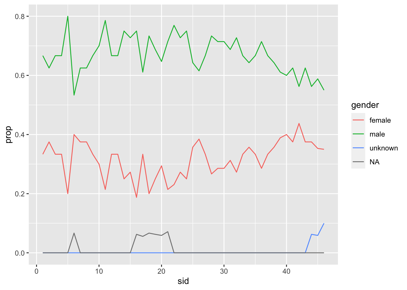

The plot looks good, but let’s do some more customizing.

ggplot(casts_prop_all,aes(sid,prop,col=gender))+
  geom_path()+
  scale_y_continuous(limits=c(0,1))+
  scale_color_discrete(name="Gender")+
  labs(x="Season",
       y="Proportion",
       title="Saturday Night Live",
       subtitle="Gender Makeup by Season")+
  ggthemes::theme_few()+
  theme(plot.title = element_text(hjust=0.5),
        plot.subtitle=element_text(hjust=0.5))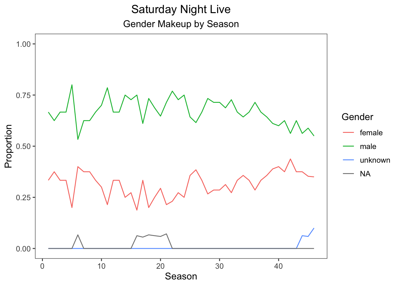

It looks like over the years, the gender makeup has slightly trended towards equality, but we are far from full equality in SNL.

One more note: the reader may have a hard time contextualizing these data in terms of “Season Number”. It may be more helpful to plot these data in terms of the YEAR the season aired. To do that, we need to use left_join() to combine our data with the seasons dataframe.

casts_prop_all %>%
  left_join(seasons,by="sid") %>%
  mutate(year=lubridate::ymd(year,truncated=4)) %>%
  ggplot(aes(year,prop,col=gender))+
  geom_path()+
  scale_x_date(date_labels="%Y",breaks = "5 years")+
  scale_y_continuous(limits=c(0,1))+
  scale_color_discrete(name="Gender")+
  labs(x="Year",
       y="Proportion",
       title="Saturday Night Live",
       subtitle="Gender Makeup by Year")+
  ggthemes::theme_few()+
  theme(plot.title = element_text(hjust=0.5),
        plot.subtitle=element_text(hjust=0.5),
        axis.text.x = element_text(angle=90))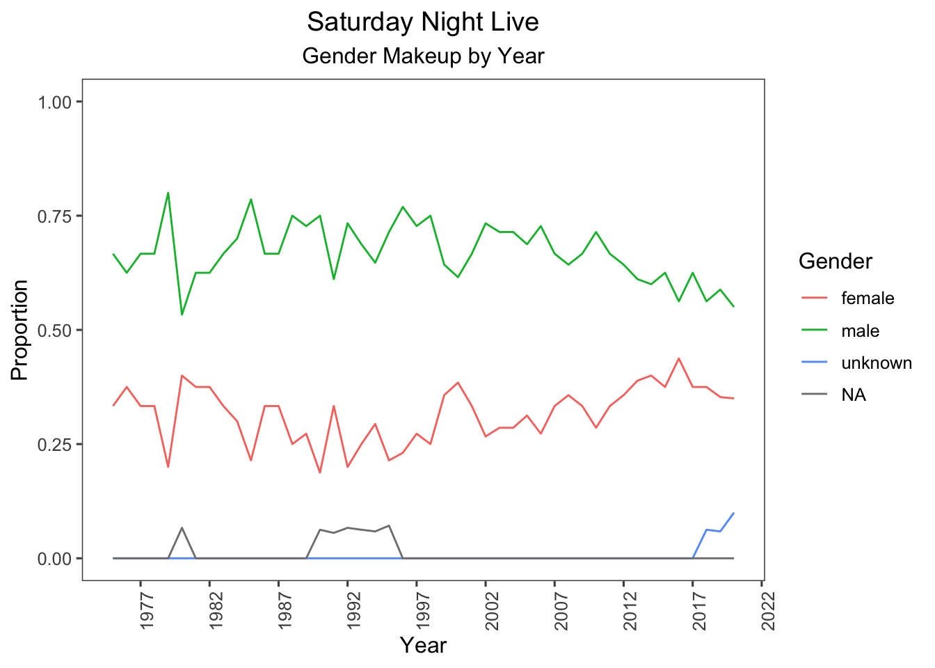

That’s better. This way, the reader can contextualize the data easier.

More analysis/visualization

We might also consider analyzing the male/non-male ratio over the years, to get an idea of the magnitude of gender bias in the way a proportion might not give us. To do so, we use pivot_wider(), mutate(), replace_na(), and left_join() again to get a measure of \(\frac{male}{nonmale}\) ratio over the years. We again use geom_path() to plot this ratio over the years. We also use geom_hline() to plot a horizontal line where \(\frac{male}{nonmale}\) ratio equals 1.¹

casts_gender_count %>%
  pivot_wider(names_from = gender,
              values_from = n) %>% 
  mutate(across(c(`NA`,unknown,male,female),~replace_na(.,0)),
         male_nonmale_ratio=male/(female+unknown+`NA`)) %>%
  left_join(seasons,by="sid") %>%
  mutate(year=lubridate::ymd(year,truncated=4)) %>%
  ggplot(aes(year,male_nonmale_ratio))+
  geom_path(col="dodgerblue3")+
  geom_hline(yintercept=1,col="red",linetype="dashed")+
  scale_x_date(date_labels="%Y",breaks = "5 years")+
  scale_y_continuous(limits=c(0,5))+
  labs(x="Year",
       y="Male/Non-Male Ratio",
       title="Saturday Night Live",
       subtitle="Male Bias Over the Years")+
  theme_classic()+
  theme(plot.title=element_text(hjust=0.5),
        plot.subtitle=element_text(hjust=0.5))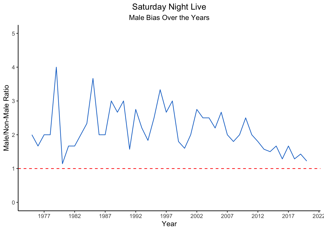

Again, it looks like there’s been a consistent male bias over the years, which, although trending downward, does not suggest we are at any sort of equality/representation in entertainment.

Conclusion

We’ve managed to put together a relatively straightforward analysis & visualization of the gender makeup of Saturday Night Live over the years. A more complex analysis might also take into account the number of sketches cast members of each gender performed in over the years.

In addition, there are numerous other demographic variables not currently taking into consideration that might provide a more complete analysis of representation in the entertainment industry.

With that being said, this relatively simple analysis is intended to be pedagogical in nature, as a way to demonstrate further some of the helpful data analysis tools available in dplyr, tidyr, and ggplot2.

Footnotes

1. Note: A male/non-male ratio of 1 does NOT indicate a lack of gender bias, as the full spectrum of gender is not represented at all in these data. Rather, it indicates a lack of bias in favor of males when compared with the combined sum of all other genders currently available in the data. That is, a value of 1 is not evidence in favor of gender equality in the data.