Challenge 8

challenge_8

Prasann Desai

snl

Joining Data

Author

Prasann Desai

Published

July 3, 2023

library(tidyverse)
library(ggplot2)
library(readxl)
library(lubridate)
library(scales)

knitr::opts_chunk$set(echo = TRUE, warning=FALSE, message=FALSE)

Challenge Overview

Today’s challenge is to:

read in multiple data sets, and describe the data set using both words and any supporting information (e.g., tables, etc)
tidy data (as needed, including sanity checks)
mutate variables as needed (including sanity checks)
join two or more data sets and analyze some aspect of the joined data

(be sure to only include the category tags for the data you use!)

Read in data

Read in one (or more) of the following datasets, using the correct R package and command.

military marriages ⭐⭐
faostat ⭐⭐
railroads ⭐⭐⭐
fed_rate ⭐⭐⭐
debt ⭐⭐⭐
us_hh ⭐⭐⭐⭐
snl ⭐⭐⭐⭐⭐

snl_seasons <- read_csv('_data/snl_seasons.csv')
snl_actors <- read_csv('_data/snl_actors.csv')
snl_casts <- read_csv('_data/snl_casts.csv')

Previewing the datasets

# snl_casts
nrow(snl_casts)

[1] 614

head(snl_casts)

# A tibble: 6 × 8
  aid                sid featured first_epid last_epid update_…¹ n_epi…² seaso…³
  <chr>            <dbl> <lgl>         <dbl>     <dbl> <lgl>       <dbl>   <dbl>
1 A. Whitney Brown    11 TRUE       19860222        NA FALSE           8   0.444
2 A. Whitney Brown    12 TRUE             NA        NA FALSE          20   1    
3 A. Whitney Brown    13 TRUE             NA        NA FALSE          13   1    
4 A. Whitney Brown    14 TRUE             NA        NA FALSE          20   1    
5 A. Whitney Brown    15 TRUE             NA        NA FALSE          20   1    
6 A. Whitney Brown    16 TRUE             NA        NA FALSE          20   1    
# … with abbreviated variable names ¹update_anchor, ²n_episodes,
#   ³season_fraction

# snl_seasons
nrow(snl_seasons)

[1] 46

head(snl_seasons)

# A tibble: 6 × 5
    sid  year first_epid last_epid n_episodes
  <dbl> <dbl>      <dbl>     <dbl>      <dbl>
1     1  1975   19751011  19760731         24
2     2  1976   19760918  19770521         22
3     3  1977   19770924  19780520         20
4     4  1978   19781007  19790526         20
5     5  1979   19791013  19800524         20
6     6  1980   19801115  19810411         13

# snl_actors
nrow(snl_actors)

[1] 2306

head(snl_actors)

# A tibble: 6 × 4
  aid            url           type  gender 
  <chr>          <chr>         <chr> <chr>  
1 Kate McKinnon  /Cast/?KaMc   cast  female 
2 Alex Moffat    /Cast/?AlMo   cast  male   
3 Ego Nwodim     /Cast/?EgNw   cast  unknown
4 Chris Redd     /Cast/?ChRe   cast  male   
5 Kenan Thompson /Cast/?KeTh   cast  male   
6 Carey Mulligan /Guests/?3677 guest andy

Briefly describe the data

From the above outputs, we can see that the dataset contains 3 tables related to the popular show (SNL- Saturday Night Live). - snl_actors contains a list of actors who appeared on SNL with a few characterstics about them like their url, gender and whether they were a cast/guest/crew/unknown member on SNL. - snl_seasons contains a list of SNL seasons and basic information about it like first/last episode ids, num of episodes and year of the SNL season. - snl_casts contains the details of actors that featured in every season of SNL and their stats like num of episodes they were part of, their first/last episode ids, etc.

Tidy Data (as needed)

Is your data already tidy, or is there work to be done? Be sure to anticipate your end result to provide a sanity check, and document your work here.

Response: Overall, all the 3 tables look tidy.

Are there any variables that require mutation to be usable in your analysis stream? For example, do you need to calculate new values in order to graph them? Can string values be represented numerically? Do you need to turn any variables into factors and reorder for ease of graphics and visualization?

Document your work here.

table(snl_actors$gender)


   andy  female    male unknown 
     21     671    1226     388

# SNL actors dataset contains 'andy' gender. It would be a good idea to replace these instances with 'unknown'.
snl_actors <- mutate(snl_actors, gender = case_when(str_detect(gender, "andy") ~ "unknown",
                                                    str_equal(gender, "female") ~ "female",
                                                    str_equal(gender, "male") ~ "male",
                                                    TRUE ~ as.character(gender)
                                                    ))
# Sanity check of the fix
table(snl_actors$gender)


 female    male unknown 
    671    1226     409

Join Data

Be sure to include a sanity check, and double-check that case count is correct!

# Joining the snl_casts and snl_actors on "aid" column
snl_ca <- left_join(snl_casts, snl_actors, by = "aid")
snl_ca

# A tibble: 614 × 11
   aid           sid featu…¹ first…² last_…³ updat…⁴ n_epi…⁵ seaso…⁶ url   type 
   <chr>       <dbl> <lgl>     <dbl>   <dbl> <lgl>     <dbl>   <dbl> <chr> <chr>
 1 A. Whitney…    11 TRUE     1.99e7      NA FALSE         8   0.444 /Cas… cast 
 2 A. Whitney…    12 TRUE    NA           NA FALSE        20   1     /Cas… cast 
 3 A. Whitney…    13 TRUE    NA           NA FALSE        13   1     /Cas… cast 
 4 A. Whitney…    14 TRUE    NA           NA FALSE        20   1     /Cas… cast 
 5 A. Whitney…    15 TRUE    NA           NA FALSE        20   1     /Cas… cast 
 6 A. Whitney…    16 TRUE    NA           NA FALSE        20   1     /Cas… cast 
 7 Alan Zweib…     5 TRUE     1.98e7      NA FALSE         5   0.25  /Cas… cast 
 8 Sasheer Za…    39 TRUE     2.01e7      NA FALSE        11   0.524 /Cas… cast 
 9 Sasheer Za…    40 TRUE    NA           NA FALSE        21   1     /Cas… cast 
10 Sasheer Za…    41 FALSE   NA           NA FALSE        21   1     /Cas… cast 
# … with 604 more rows, 1 more variable: gender <chr>, and abbreviated variable
#   names ¹featured, ²first_epid, ³last_epid, ⁴update_anchor, ⁵n_episodes,
#   ⁶season_fraction

# Joining the snl_ca and snl_seasons on "sid" column
snl_cas <- left_join(snl_ca, snl_seasons, by = "sid")
snl_cas

# A tibble: 614 × 15
   aid           sid featu…¹ first…² last_…³ updat…⁴ n_epi…⁵ seaso…⁶ url   type 
   <chr>       <dbl> <lgl>     <dbl>   <dbl> <lgl>     <dbl>   <dbl> <chr> <chr>
 1 A. Whitney…    11 TRUE     1.99e7      NA FALSE         8   0.444 /Cas… cast 
 2 A. Whitney…    12 TRUE    NA           NA FALSE        20   1     /Cas… cast 
 3 A. Whitney…    13 TRUE    NA           NA FALSE        13   1     /Cas… cast 
 4 A. Whitney…    14 TRUE    NA           NA FALSE        20   1     /Cas… cast 
 5 A. Whitney…    15 TRUE    NA           NA FALSE        20   1     /Cas… cast 
 6 A. Whitney…    16 TRUE    NA           NA FALSE        20   1     /Cas… cast 
 7 Alan Zweib…     5 TRUE     1.98e7      NA FALSE         5   0.25  /Cas… cast 
 8 Sasheer Za…    39 TRUE     2.01e7      NA FALSE        11   0.524 /Cas… cast 
 9 Sasheer Za…    40 TRUE    NA           NA FALSE        21   1     /Cas… cast 
10 Sasheer Za…    41 FALSE   NA           NA FALSE        21   1     /Cas… cast 
# … with 604 more rows, 5 more variables: gender <chr>, year <dbl>,
#   first_epid.y <dbl>, last_epid.y <dbl>, n_episodes.y <dbl>, and abbreviated
#   variable names ¹featured, ²first_epid.x, ³last_epid.x, ⁴update_anchor,
#   ⁵n_episodes.x, ⁶season_fraction

Data Analysis

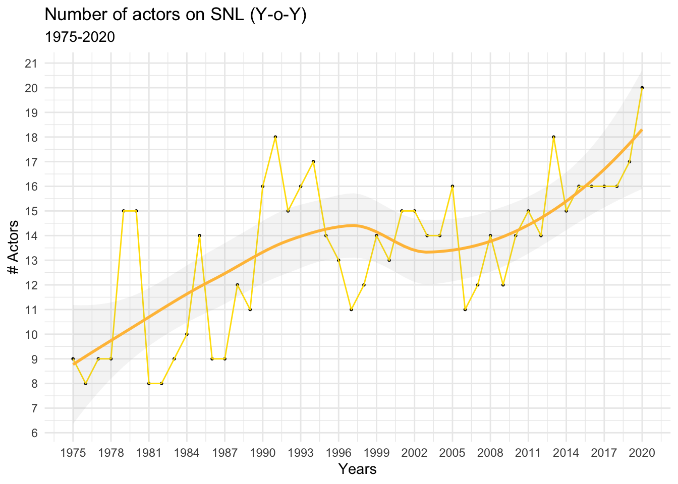
snl_actors_years <- select(snl_cas, aid, year)
snl_yoy_actors <- count(snl_actors_years, year)
snl_yoy_actors <- mutate(snl_yoy_actors, 
                       year = as.Date(paste0(as.character(year), "0101"),format = "%Y%m%d"))
snl_yoy_actors

# A tibble: 46 × 2
   year           n
   <date>     <int>
 1 1975-01-01     9
 2 1976-01-01     8
 3 1977-01-01     9
 4 1978-01-01     9
 5 1979-01-01    15
 6 1980-01-01    15
 7 1981-01-01     8
 8 1982-01-01     8
 9 1983-01-01     9
10 1984-01-01    10
# … with 36 more rows

# Line plot of trend of number of actors on SNL over years

#debt_pivoted$year_q <- yq(paste0(debt_pivoted$Year, ":", debt_pivoted$Quarter))

ggplot(snl_yoy_actors, aes(x = year, y = n)) +
  geom_point(size=0.5) +
  geom_line(size=0.5, color = "#FFDF00") +
  geom_smooth(alpha = 0.1, color = "#FFBF46") + 
  scale_x_date(date_breaks = '3 years',
               labels = date_format("%Y")) +
  scale_y_continuous(breaks = c(seq(1, 25, by=1))) +
  labs(title = "Number of actors on SNL (Y-o-Y)",
       subtitle = "1975-2020",
       x = "Years",
       y = "# Actors") +
  theme_minimal() +
  scale_color_brewer(palette = "Dark2")