Challenge 5

challenge_5

air_bnb

Introduction to Visualization

Author

Danny Holt

Published

June 15, 2023

library(tidyverse)
library(ggplot2)

knitr::opts_chunk$set(echo = TRUE, warning=FALSE, message=FALSE)

Read in data

Read in - AB_NYC_2019.csv ⭐⭐⭐

abnb <- readr::read_csv("_data/AB_NYC_2019.csv")
abnb

glimpse(abnb)

Rows: 48,895
Columns: 16
$ id                             <dbl> 2539, 2595, 3647, 3831, 5022, 5099, 512…
$ name                           <chr> "Clean & quiet apt home by the park", "…
$ host_id                        <dbl> 2787, 2845, 4632, 4869, 7192, 7322, 735…
$ host_name                      <chr> "John", "Jennifer", "Elisabeth", "LisaR…
$ neighbourhood_group            <chr> "Brooklyn", "Manhattan", "Manhattan", "…
$ neighbourhood                  <chr> "Kensington", "Midtown", "Harlem", "Cli…
$ latitude                       <dbl> 40.64749, 40.75362, 40.80902, 40.68514,…
$ longitude                      <dbl> -73.97237, -73.98377, -73.94190, -73.95…
$ room_type                      <chr> "Private room", "Entire home/apt", "Pri…
$ price                          <dbl> 149, 225, 150, 89, 80, 200, 60, 79, 79,…
$ minimum_nights                 <dbl> 1, 1, 3, 1, 10, 3, 45, 2, 2, 1, 5, 2, 4…
$ number_of_reviews              <dbl> 9, 45, 0, 270, 9, 74, 49, 430, 118, 160…
$ last_review                    <date> 2018-10-19, 2019-05-21, NA, 2019-07-05…
$ reviews_per_month              <dbl> 0.21, 0.38, NA, 4.64, 0.10, 0.59, 0.40,…
$ calculated_host_listings_count <dbl> 6, 2, 1, 1, 1, 1, 1, 1, 1, 4, 1, 1, 3, …
$ availability_365               <dbl> 365, 355, 365, 194, 0, 129, 0, 220, 0, …

Briefly describe the data

The data has 16 variables/columns and 48,895 rows. The data shows Airbnb rental listings in New York City during 2019. Each listing includes:

id: unique numerical ID

name: listing title

host_id: host’s unique numerical ID

host_name: listed name(s) of host(s)

neighbourhood_group: the borough of New York City where the listing is

distinct(abnb,neighbourhood_group)

neighbourhood: the neighborhood (below the borough level) where the listing is

latitude: the latitude coordinate of the listing

longitude: the longitude coordinate of the listing

room_type: the type of listing

distinct(abnb,room_type)

price: price per night

minimum_nights: minimum number of nights possible to rent

number_of_reviews: number of visitor reviews

last_review: date of most recent review

reviews_per_month: number of reviews written per month

calculated_host_listings_count: number of total listings the host has on Airbnb

availability_365: number of nights the listing is available to rent per year

Tidy Data (as needed)

The data is already tidy. Each variable has its own column and each observation (listing) has its own row.

But, let’s mutate some categorical variables into factors for later on.

abnb <- abnb %>%
  mutate(neighbourhood_group = as_factor(neighbourhood_group),
    neighbourhood = as_factor(neighbourhood),
    room_type = as_factor(room_type))

Univariate Visualizations

Let’s look at a bar chart of room types of listings. This chart type is a good choice because room_type is categorical.

ggplot(abnb, aes(room_type)) +
  geom_bar() +
  labs(title = "Number of NYC Airbnb listings by type, 2019", x = "Listing type", y = "Amount") +
  theme_bw()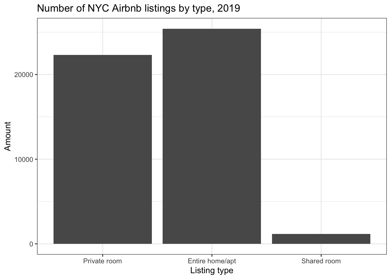

Now, let’s look at a histogram of prices. This is a good choice to show the distribution of a single numerical variable like price. First, though, we’ll filter out outliers with prices at or above $2000/night to make the graph easier to understand.

abnb %>%
  filter(price < 1500) %>%
  ggplot(aes(price)) +
    geom_histogram() +
    labs(title = "Nightly prices of NYC Airbnb listings, 2019", x = "Nightly price, $", y = "Amount of listings") +
    theme_bw()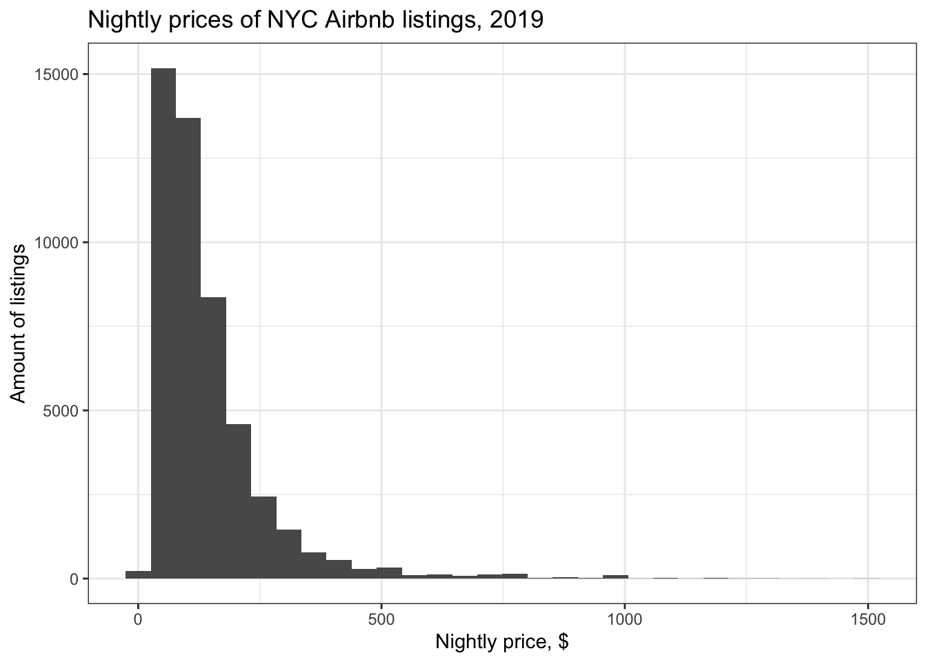

Bivariate Visualization

Now, let’s look at a bivariate visualization. We can see if there’s a relationship between price and minimum_nights. We’ll use a scatter plot, which is good for looking at relationships between two numeric variables.

abnb %>%
  ggplot(aes(x=price,y=minimum_nights)) +
  geom_point() +
  geom_smooth() +
  labs(title="Price vs. Night Minimum of NYC Airbnb listings, 2019",x="Nightly price, $",y="Minimum # of nights allowed to rent") +
  theme_bw()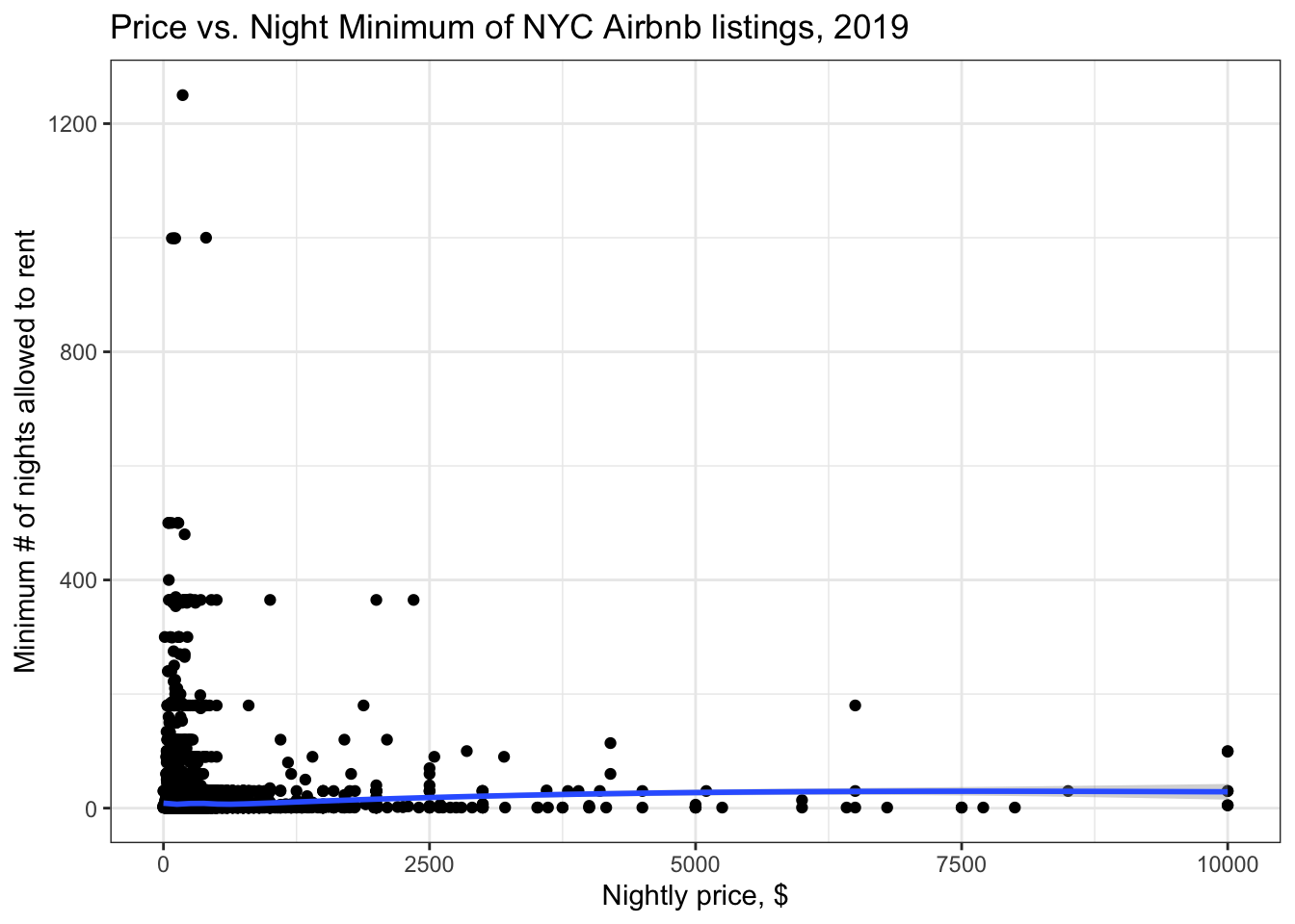

Let’s see if this gets better when we filter out listings with unusually high prices.

abnb %>%
  filter(price<600) %>%
  ggplot(aes(x=price,y=minimum_nights)) +
  geom_point() +
  geom_smooth() +
  labs(title="Price vs. Night Minimum of NYC Airbnb listings, 2019",x="Nightly price, $",y="Minimum # of nights allowed to rent") +
  theme_bw()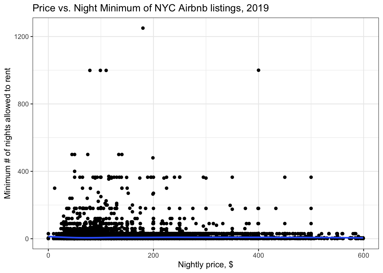

It still looks like there’s not much of a link.