Challenge 8

Joining Data

Code

library(tidyverse)
library(ggplot2)
library(readxl)

knitr::opts_chunk$set(echo = TRUE, warning=FALSE, message=FALSE)

Read in data

For this challenge, I will be using two sets of economic data: the debt and fed_rate datasets.

Code

# read in debt
debt <- read_excel("_data/debt_in_trillions.xlsx")
debt

Code

# read in fed rate
fed <- read_csv("_data/FedFundsRate.csv")
fed

Briefly describe the data

Debt

The data shows quarterly measures (in trillions of dollars) of debt associated with six types of loans: Mortgage, HE Revolving, Auto Loan Credit Card, Student Loan, and Other (plus a Total).

The data runs from the start of 2003 through the second quarter of 2021.

Fed rate

This data includes economic information like GDP, inflation, unemployment, and federal funds rates.

The data runs from July 1, 1954 to March 16, 2017.

Tidy Data

Are there any variables that require mutation to be usable in your analysis stream? For example, do you need to calculate new values in order to graph them? Can string values be represented numerically? Do you need to turn any variables into factors and reorder for ease of graphics and visualization?

Debt

The data is mostly tidy, though we need to adjust the format in which dates are presented. We’ll use mutate() and parse_date_time() to create a Date column with proper date formatting.

Code

# use parse_date_time to parse out dates from years and quarters
debt <- debt %>%
  mutate(Date=parse_date_time(`Year and Quarter`,
                              orders="yq"))
# remove `Year and Quarter` column
debt <- debt %>%
  select(-one_of("Year and Quarter")) %>%
  # move Date to front
  select(Date, everything())
# view data
debt

We’re also going to create an alternate pivoted version of the data frame in which each observation contains data for a single type of debt with a date and amount. This version will have columns Date, Type, and Amount.

Code

debt_longer<- debt %>%
  pivot_longer(cols=c(`Mortgage`,`HE Revolving`,`Auto Loan`,`Credit Card`,`Student Loan`,`Other`), names_to = "Type", values_to = "Amount")
debt_longer<-debt_longer %>%
  select(Date,Type,Amount)
debt_longer

Fed rate

The data is mostly tidy. We’ll just want to change how dates are shown. Let’s create a date column out columns with year, month, and day data.

Code

#create date column out of original columns
fed_date <- paste(fed$Year, fed$Month, fed$Day)
# mutate new column
fed <- fed %>%
  mutate(Date = as.Date(fed_date,format = "%Y %m %d"), .before=`Year`)
# filter out old date rows
fed <- fed[-c(2, 3, 4)]
fed

Join Data

Because the fed data extends far before the debt data, I am choosing to use right_join() to use only data with dates matching those in debt.

Code

combined <- fed %>%
  right_join(debt, by=join_by(Date)) %>%
  rename(OtherDebt=Other,TotalDebt=Total)
combined

Code

# filter date so data is present for both sets
combined <- combined %>%
  filter(Date < '2017-01-01')
combined

Analysis

Let’s create a couple of functions and columns to view percent change in total debt acquisition. This will be useful for a comparison with percent change in GDP

Code

# create percent change function
pct <- function(x) {
  (x - lag(x))/lag(x)
}

# create change function so we can view debt acquisition rather than total debt
chg <- function(x) {
  x - lag(x)
}

# create a new column for debt acquisition and another for percent change in debt acquisition 
combined <- combined %>%
  mutate(debt_ac=chg(TotalDebt)) %>%
  mutate(chg_debt_ac = pct(debt_ac))

Now, let’s plot percent change in debt acquisition relative to percent change in GDP.

Code

# plot
ggplot(combined, aes(x=`Real GDP (Percent Change)`,y=`chg_debt_ac`)) +
  geom_point() +
  labs(title="Change in GDP and Debt Acquisition",subtitle="2003 - 2016",y="(%) Total Debt Acquisition",x="(%) GDP") +
  xlim(-3,6) +
  ylim(-3,3) +
  theme_minimal()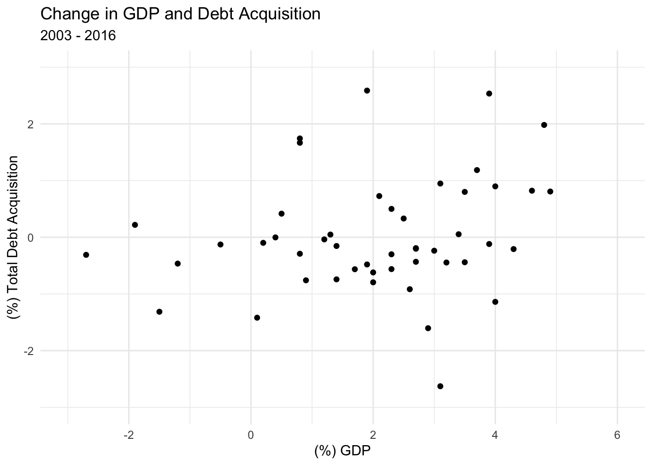

Now, let’s use a bivariate linear model to examine the relationship.

Code

# bivariate linear model
cor(combined$`Real GDP (Percent Change)`, combined$chg_debt_ac, use="pairwise.complete.obs")

[1] -0.07883687