Final Project

Final

strikes

Author

Danny Holt

Published

July 13, 2023

Code

library(tidyverse)
library(readxl)

knitr::opts_chunk$set(echo = TRUE, warning=FALSE, message=FALSE)

Introduction

In this project, I will examine data on labor strikes in the United States over the past thirty years. My goal here is to gain a better understanding of the contemporary labor movement in the U.S. by looking at changes in its most significant activity—strikes.

For those who may not know, a strike occurs when workers collectively protest by withholding their labor. Typically, after authorization through a vote within their union, workers provide notice to their employer before halting work and forming picket lines, aiming to pressure the employer into meeting their demands. The strike usually concludes when an agreement is reached between the two sides.

By examining trends in strikes, we can get a better sense of ebbs and flows in militancy in the American labor movement. In the context of the labor movement, “militancy” refers to workers’ and unions’ aggressiveness in pursuing their goals. It represents a willingness to engage in protests, strikes, and other forms of action, meant to apply pressure on employers and demonstrate collective power.

Description of the data

This dataset, monthly-listing.xlsx, shows data on work stoppages (strikes) from the Bureau of Labor Statistics, part of the U.S. Department of Labor, from 1993 to 2023 (Bureau of Labor Statistics 2023a). Each case represents a distinct strike. Workers under Work Stoppages program of the Bureau of Labor Statistics track all strikes in the U.S.

Code

# First, we'll read in the data from the Excel sheet `monthly-listing.xlsx`.

  # read in data
  strike <- read_excel("_data/monthly-listing.xlsx", skip=1)

  # filter out footnotes
  strike <- head(strike, -6)

# Next, we'll clean the data. First, we'll remove redundant and unnecessary variables. Then, we'll rename some variables with cumbersome or confusing titles.

  # remove redundant and unnecessary variables
  strike <- strike %>%
    select("Organizations involved","States","Areas","Ownership","Union acronym","Work stoppage beginning date","Work stoppage ending date","Number of workers[2]","Days idle, cumulative for this work stoppage[3]")

  # rename variables
  strike <- strike %>%
    rename(
      "Employer"="Organizations involved",
      "Union"="Union acronym",
      "Start date"="Work stoppage beginning date",
      "End date"="Work stoppage ending date",
      "Workers"="Number of workers[2]",
      "Days struck"="Days idle, cumulative for this work stoppage[3]"
    )

# view data
strike

Code

# view number of rows
nrow(strike)

[1] 629

There are 629 rows in the cleaned dataset, representing 629 strikes.

Variables

`Employer`

Shows the employer of the workers striking. This variable is categorical.

Code

# number of distinct employers
n_distinct(strike$Employer)

[1] 485

There are 485 distinct employers in the dataset.

Here are some of the employers with the most strikes in the period:

Code

# create factor levels (by occurrences)
em_levels = names(sort(table(strike$Employer), decreasing = TRUE))

# view
head(em_levels)

[1] "General Motors Corp."     "Kaiser Permanente"       
[3] "University of California" "Boeing Company"          
[5] "Caterpillar, Inc."        "Sutter Health Hospitals"

Let’s visualize the frequency.

Code

# count strikes per employer
count_em <- table(strike$Employer)
count_em_df <- data.frame(NumStrikes = as.numeric(names(count_em)),
                               Count = as.numeric(count_em))
#TEST
ggplot(count_em_df,aes(Count)) +
  geom_histogram() +
  labs(title="Distribution of employers by number of strikes",x="# of strikes",y="# of employers") +
  theme_minimal()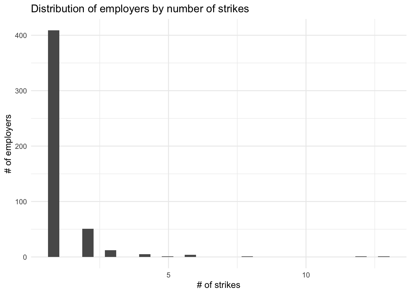

We can see that a few employers were struck many times, but most were only struck one or two times.

If we dig deeper, we can see that most employers with many strikes were struck by multiple different unions. One thing this can signal is a high level of militancy across different types of workers employed by the employer. For instance, an employer like the University of California, which had the third-most strikes in the period, employs many different types of workers belonging to different unions, including CWA, the UAW, AFSCME, and the IBT. See here:

Code

strike %>%
  filter(Employer == "University of California")

However, the presence of strikes by multiple unions at a single employer can also signal turf disputes. This is the case with Kaiser Permanente, the employer with the second-most strikes in the period, which saw strikes from separate healthcare workers’ unions, including SEIU, CNA, and NUHW (in addition to UFCW, which represents non-healthcare workers). See here:

Code

strike %>%
  filter(Employer == "Kaiser Permanente")

`States`

Shows the state or state(s) in which the strike took place. This variable is categorical.

Code

# break out entries with multiple states
strike_st <- separate_rows(strike,States,sep=", ")
strike_st <- separate_rows(strike_st,States,sep=",")

# filter out data without valid state information
strike_st <- strike_st %>%
  filter(!grepl("Interstate", States)) %>%
  filter(!grepl("East Coast States", States)) %>%
  filter(!grepl("Nationwide", States))

# convert states to factors
st_levels <- c("WY", "WI", "WV", "WA", "VA", "VT", "UT", "TX", "TN", "SD", "SC", "RI", "PA", "OR", "OK", "OH", "ND", "NC", "NY", "NM", "NJ", "NH", "NV", "NE", "MT", "MO", "MS", "MN", "MI", "MA", "MD", "ME", "LA", "KY", "KS", "IA", "IN", "IL", "ID", "HI", "GA", "FL", "DE", "CT", "CO", "CA", "AR", "AZ", "AK", "AL")
strike_st <- strike_st %>%
  mutate(States=factor(States,levels=st_levels))

# drop NA
strike_st <- strike_st %>%
  drop_na(States)

Let’s look at the frequency of strikes across the states. Here is a visualization:

Code

# visualize frequency
strike_st %>%
  count(States) %>%
  ggplot(aes(reorder(States,n),n)) +
  geom_col() +
  coord_flip() +
  scale_x_discrete(guide = guide_axis(n.dodge=1)) +
  theme_minimal() +
  labs(title="Number of strikes by state",subtitle="1993 - 2023",x="State",y="# of strikes")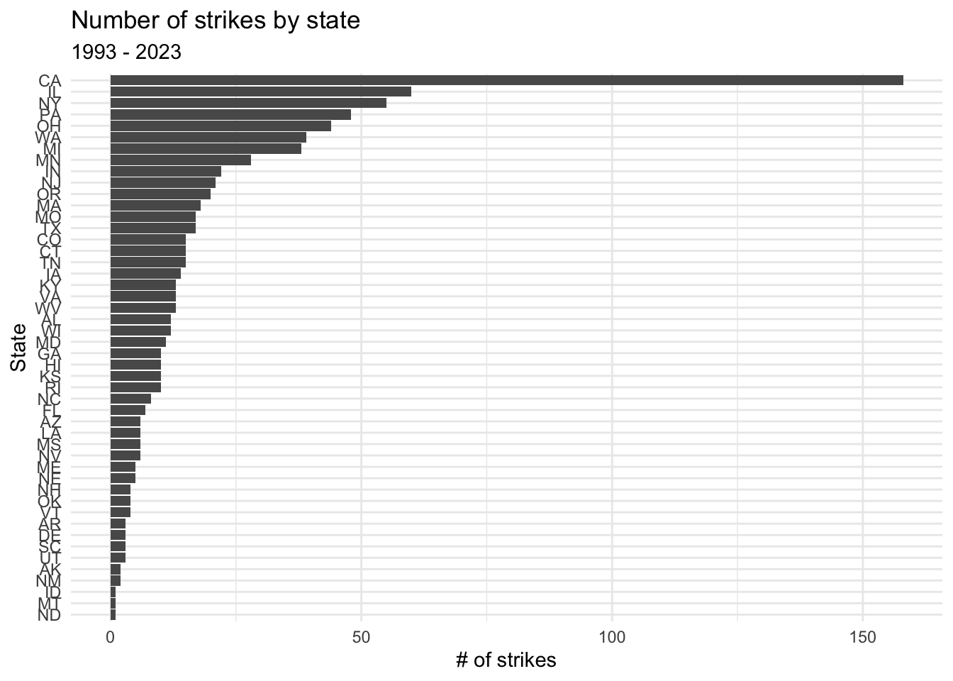

We can see that the states with the most strikes in the period are: California, Illinois, New York, Pennsylvania, Ohio, and Washington. This makes perfect sense, based on the economic and political conditions of those states. Illinois, Pennsylvania, and Ohio are all home to large automotive and other manufacturing unions. Meanwhile, California, New York, and Washington all have high union density overall, with long and storied histories of labor activism. Additionally, all six of these states have above-average populations.

`Areas`

Shows a more specific location of the strike, at a lower level than the state(s). This variable is categorical.

Because the areas are written to be geographically overlapping and range in size from cities to entire regions, the frequency information for this variable is relatively meaningless.

`Ownership`

Shows what type of entity the employer is of the following options: private industry, local and/or state government. This variable is categorical.

Let’s visualize the frequency of ownership types in strikes.

Code

# break out state and local government into state government and local government,
strike_own <- separate_rows(strike,Ownership,sep=" and ")
strike_own <- strike_own %>%
  mutate(Ownership=case_when(
    Ownership == "State" ~ "State government",
    Ownership == "State government" ~ "State government",
    Ownership == "Local government" ~ "Local government",
    Ownership == "local government" ~ "Local government",
    Ownership == "Private industry" ~ "Private industry"),
    )

# filter out data without valid information
strike_own <- strike_own %>%
  drop_na(Ownership)

# convert ownership types to factors
own_levels <- c("Private industry", "State government", "Local government")
strike_own <- strike_own %>%
  mutate(Ownership=factor(Ownership,levels=own_levels))

# bar graph
strike_own %>%
  count(Ownership) %>%
  ggplot(aes(reorder(Ownership,-n),n)) +
  geom_bar(stat="identity") +
  labs(title="Number of strikes by employer ownership type",subtitle="1993 - 2023",x="Ownership type",y="# of strikes") +
  theme_minimal()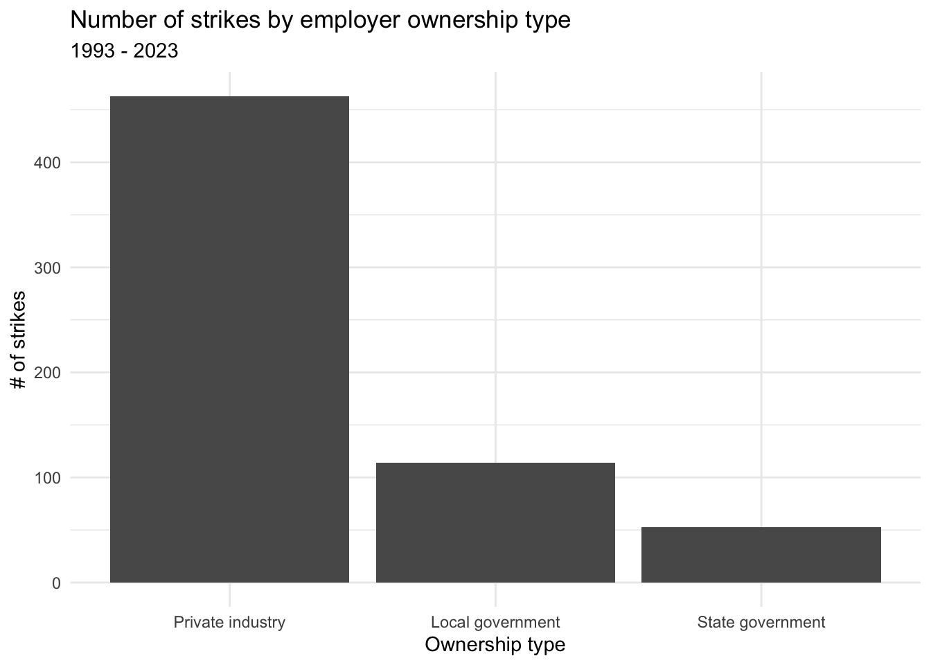

This chart shows, more than anything else, the vastness of the private sector compared with the public sector in the U.S. Indeed, the fact that the bars for local and state government strikes are as large as they are is a testament to a much higher unionization rate in the public sector than in the private sector—33.1% in the public sector versus 6.0% in the private sector (Bureau of Labor Statistics 2023b).

`Union`

Shows the acronym of the union to which the striking workers belonged. This variable is categorical.

Code

# separate cells with multiple unions
strike_un <- separate_rows(strike,Union,sep=", ")
strike_un <- separate_rows(strike_un,Union,sep="; ")
strike_un <- separate_rows(strike_un,Union,sep=". ")

# filter out separate entries for union local numbers (redundant)
strike_un <- strike_un %>%
  filter(!grepl("234", Union)) %>%
  filter(!grepl("1594", Union))

# drop NA
strike_un <- strike_un %>%
  drop_na(Union)

# create factor levels (by occurrences)
un_levels = names(sort(table(strike_un$Union), decreasing = TRUE))

# sort employers
strike_un <- strike_un %>%
  mutate(Union = factor(Union, levels=un_levels))

# number of unions
n_distinct(strike_un$Union)

[1] 131

There are 131 distinct unions in the dataset. Here are some of the Unions with the most strikes in the period:

Code

# create dataframe
top_un <- data.frame(head(un_levels))
# add full names
top_un <- top_un %>%
  mutate(Acronym=head.un_levels.) %>%
  mutate(`Full name` = case_when(
    Acronym == "SEIU" ~ "Service Employees International Union",
    Acronym == "UAW" ~ "United Auto Workers",
    Acronym == "IAM" ~ "International Association of Machinists and Aerospace Workers",
    Acronym == "IBT" ~ "International Brotherhood of Teamsters",
    Acronym == "CNA" ~ "California Nurses Association",
    Acronym == "USW" ~ "United Steelworkers"
  )) %>%
  select(`Full name`, Acronym)
# view
top_un

Let’s visualize the frequency. Because there are so many unions, I’ve chosen not to label them all for visibility reasons. Instead, I’ll sort unions from most strikes in the period to least, with a simple numerical marker. The bar for each distinct union will be colored to show distinct employers struck.

Code

# spacing for graph
spaces_un <- function(x) x[seq_along(x) %% 26 == 0]

# bar graph
ggplot(strike_un, aes(Union)) +
  geom_bar(aes(fill=Employer)) +
  labs(title="Unions in descending order of strikes",subtitle="1993 - 2023",x="Unions",y="# of strikes") +
  theme_minimal() +
  guides(fill = FALSE) +
  scale_x_discrete(breaks=spaces_un,labels=c("26","52","78","104","130"))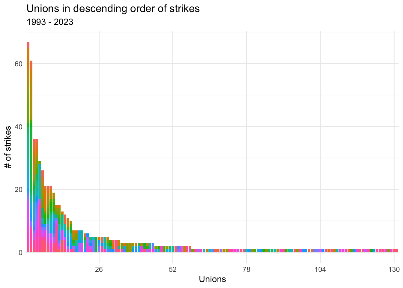

The graph shows us a few things. Perhaps most apparent is that most unions in the dataset only engaged in one strike over these three decades.

We also see that most unions with multiple strikes, like SEIU and the UAW, struck multiple employers. This may seem obvious—unions with more striking bargaining units will have more total strikes. However, the presence of strikes in one bargaining unit, I suspect, is likely to encourage action in other units (at other employers) in the same union.

`Start date` and `End date`

Start date shows the date on which the strike began. This column contains numerical, discrete, interval data.

End date shows the date on which the strike ended. This column contains numerical, discrete, interval data.

Let’s visualize the distribution of each.

Code

# pivot to create new date type variable
strike_date <- strike %>%
  pivot_longer(c(`Start date`,`End date`),names_to="Type",values_to="Date")

`Workers`

Shows the number of workers who went on strike. This column contains numerical, discrete, ratio data.

Let’s visualize the frequency with a histogram.

Code

ggplot(strike, aes(Workers)) +
  geom_histogram(binwidth=5000) +
  ggtitle("Bin size = 5000") +
  labs(title="Distribution of workers",x="Workers",y="# of strikes") +
  theme_minimal()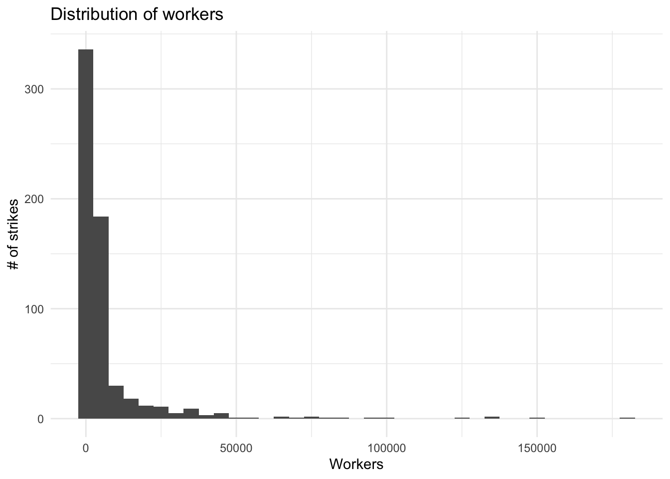

With this chart, we see that the vast majority of strikes have relatively few workers, with (generally) fewer and fewer strikes as the number of workers increases.

Let’s look at some measures of central tendency.

Code

# median
strike %>%
  summarize(Median=median(Workers, na.rm=TRUE))

Code

# mean
strike %>%
  summarize(Mean=mean(Workers, na.rm=TRUE))

Code

#std dev
strike %>%
  summarize("Standard Deviation"=sd(Workers, na.rm=TRUE))

Here, we see how the presence of many relatively small strikes brings down the median far below the mean.

`Days struck`

Shows the total number of hours of labor workers withheld during the strike. This is distinct from the difference between Start date and End date because, in some strikes, some workers go back to work before the strike ends. This column contains numerical, discrete, ratio data.

Let’s visualize the frequency with a histogram.

Code

ggplot(strike, aes(`Days struck`)) +
  geom_histogram() +
  labs(title="Distribution of days struck",y="# of strikes") +
  theme_minimal()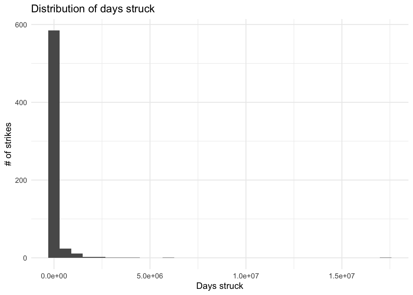

With this chart, we see that the vast majority of strikes have relatively few days struck, with (generally) fewer and fewer strikes as the number of days struck increases.

Let’s look at some measures of central tendency.

Code

# median
strike %>%
  summarize(Median=median(`Days struck`, na.rm=TRUE))

Code

# mean
strike %>%
  summarize(Mean=mean(`Days struck`, na.rm=TRUE))

Code

#std dev
strike %>%
  summarize("Standard Deviation"=sd(`Days struck`, na.rm=TRUE))

Here, we see how the presence of many relatively short and small strikes brings down the median far below the mean.

How has labor militancy changed over the past 30 years?

Measures of central tendency

To get closer to understanding how strikes and labor militancy have changed over the past three decades, we will create a new data frame, combining strikes that start in the same year and view some measures of central tendency.

Code

# select relevant variables
strike_yr <- strike %>%
  select(
    "Start date",
    "Workers",
    "Days struck",
    "Ownership",
    "States")

# truncate start date to year
strike_yr$"Start date" <- as.numeric(format(strike_yr$"Start date", "%Y"))
  
# rename start date to year
strike_yr <- strike_yr %>%
  rename("Year"="Start date") %>%
  rename("Days" = "Days struck")
  
# condense rows by year and remove problematic rows
  strike_yr_sum <- strike_yr %>%
    filter(Year>1990) %>%
    group_by(Year)
  #create condensed view
  strike_yr_sum_cond <- strike_yr_sum %>%
    summarize(
      Workers=sum(Workers, na.rm=TRUE),
      `Days Struck`=sum(Days, na.rm=TRUE),
    )
  #create less condensed view
  strike_yr_sum <- strike_yr_sum %>%
    summarize(
      Workers=sum(Workers, na.rm=TRUE),
      `Days Struck`=sum(Days, na.rm=TRUE),
      Ownership=Ownership,
      States=States
    )

For the number of workers involved in strikes each year:

Code

# median
strike_yr_sum_cond %>%
  summarize(Median=median(Workers, na.rm=TRUE))

Code

# mean
strike_yr_sum_cond %>%
  summarize(Mean=mean(Workers, na.rm=TRUE))

Code

#std dev
strike_yr_sum_cond %>%
  summarize("Standard Deviation"=sd(Workers, na.rm=TRUE))

Then, for the number of days struck each year:

Code

# median
strike_yr_sum_cond %>%
  summarize(Median=median(`Days Struck`, na.rm=TRUE))

Code

# mean
strike_yr_sum_cond %>%
  summarize(Mean=mean(`Days Struck`, na.rm=TRUE))

Code

#std dev
strike_yr_sum_cond %>%
  summarize("Standard Deviation"=sd(`Days Struck`, na.rm=TRUE))

As was the case with measures of central tendency for data on individual strikes, the medians are well below the means because of the presence of many relatively small, short strikes.

Changes in annual strike magnitude

How have numbers of workers on strike and number of days struck changed over time in the past 30 years?

Let’s view the years in order from most workers on strike to least.

Code

strike_yr_sum_cond%>%
  arrange(desc(Workers))

Next, we’ll view the years in order from most days struck to least.

Code

strike_yr_sum_cond%>%
  arrange(desc(`Days Struck`))

Let’s also visualize this. First, we’ll look at the change in workers on strike each year over time.

Code

ggplot(strike_yr_sum,aes(x=Year, y=Workers)) +
  geom_line() +
  labs(title="Change in number of striking workers by year",subtitle="1993 - 2023",x="Year",y="Workers") +
  scale_x_continuous(breaks = seq(1993,2023,by=3),
                     minor_breaks = seq(1993, 2023, by = 1)) +
  theme_minimal()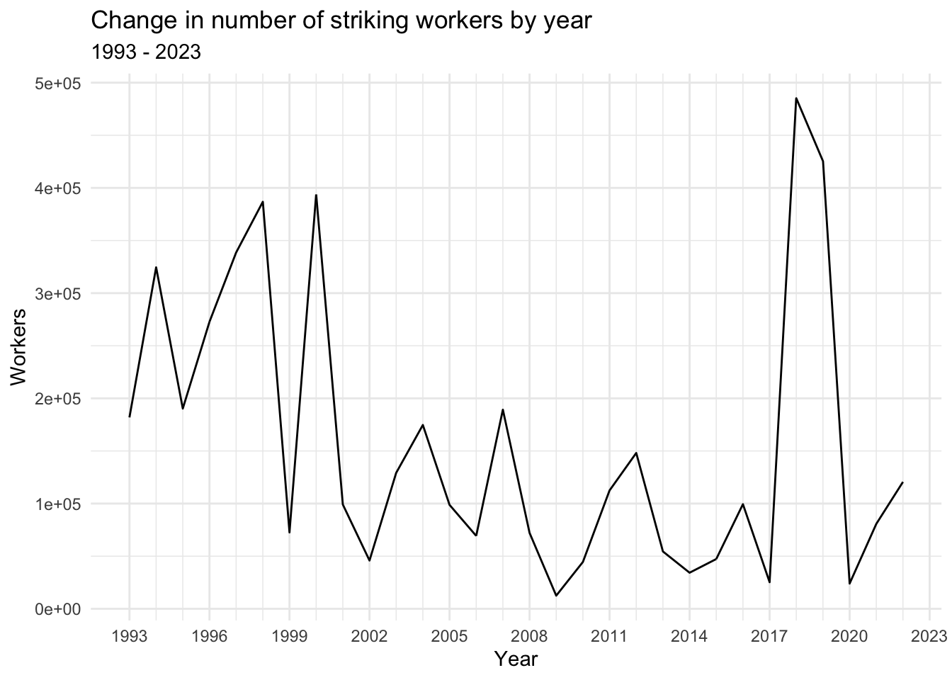

Let’s look at the same chart but, this time, with colors representing the portion of strikes with each employer ownership type.

Code

ggplot(strike_yr_sum,aes(x=Year, y=Workers,fill=Ownership)) +
  geom_area() +
  labs(title="Change in number of striking workers by year",subtitle="1993 - 2023",x="Year",y="Workers") +
  scale_x_continuous(breaks = seq(1993,2023,by=3),
                     minor_breaks = seq(1993, 2023, by = 1)) +
  theme_minimal()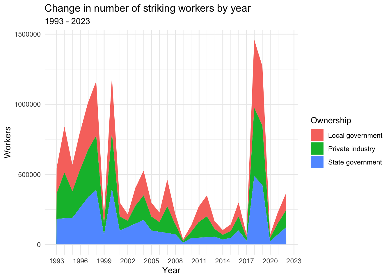

Now, we’ll take a look at the change in days struck by year.

Code

ggplot(strike_yr_sum,aes(x=Year, y=`Days Struck`)) +
  geom_line() +
  labs(title="Change in number of days struck by year",subtitle="1993 - 2023",x="Year",y="Days struck") +
  scale_x_continuous(breaks = seq(1993,2023,by=3),
                     minor_breaks = seq(1993, 2023, by = 1)) +
  theme_minimal()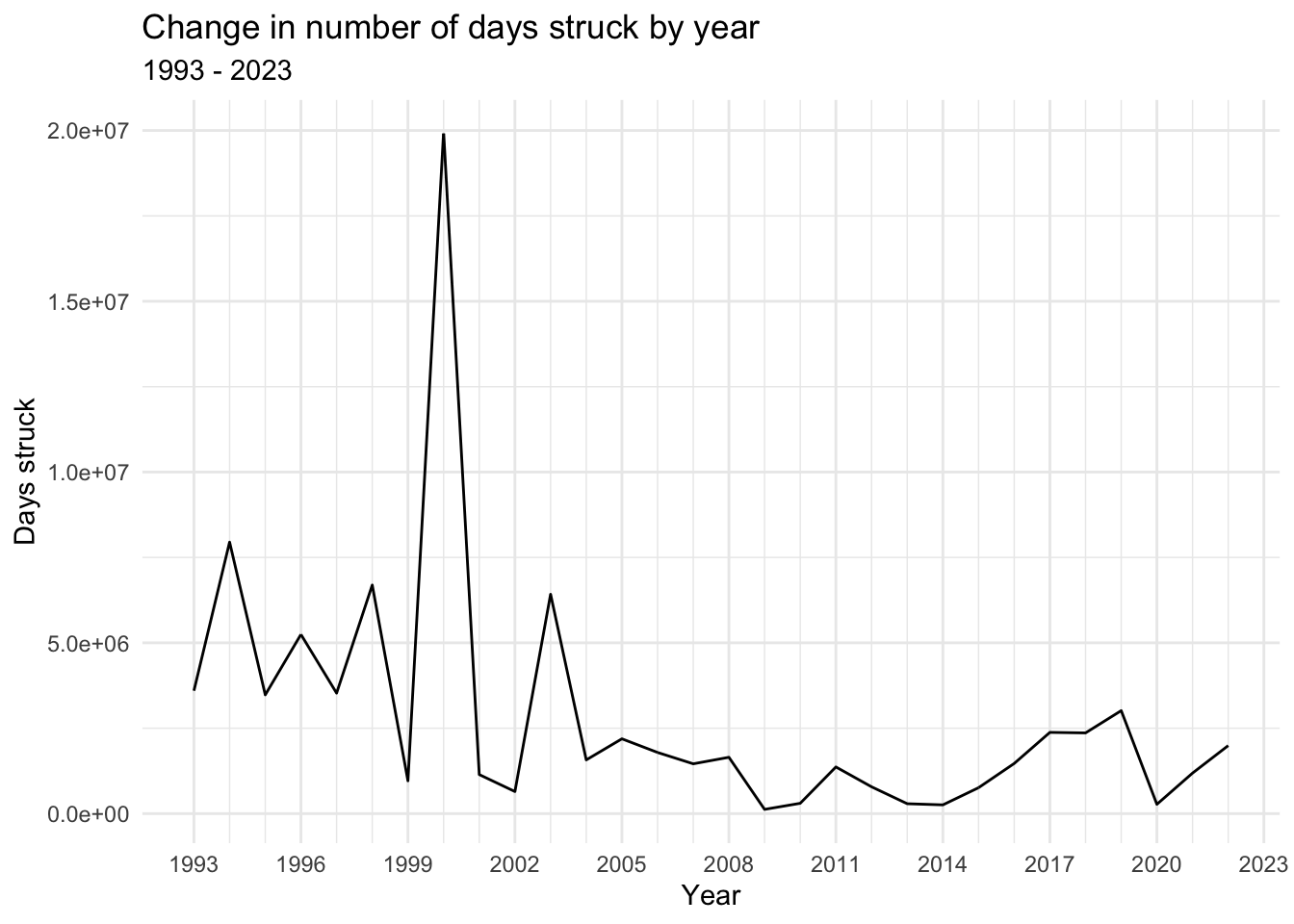

And, again, the change in days struck by year broken out by ownership type.

Code

ggplot(strike_yr_sum,aes(x=Year, y=`Days Struck`,fill=`Ownership`)) +
  geom_area() +
  labs(title="Change in number of days struck by year",subtitle="1993 - 2023",x="Year",y="Days struck") +
  scale_x_continuous(breaks = seq(1993,2023,by=3),
                     minor_breaks = seq(1993, 2023, by = 1)) +
  theme_minimal()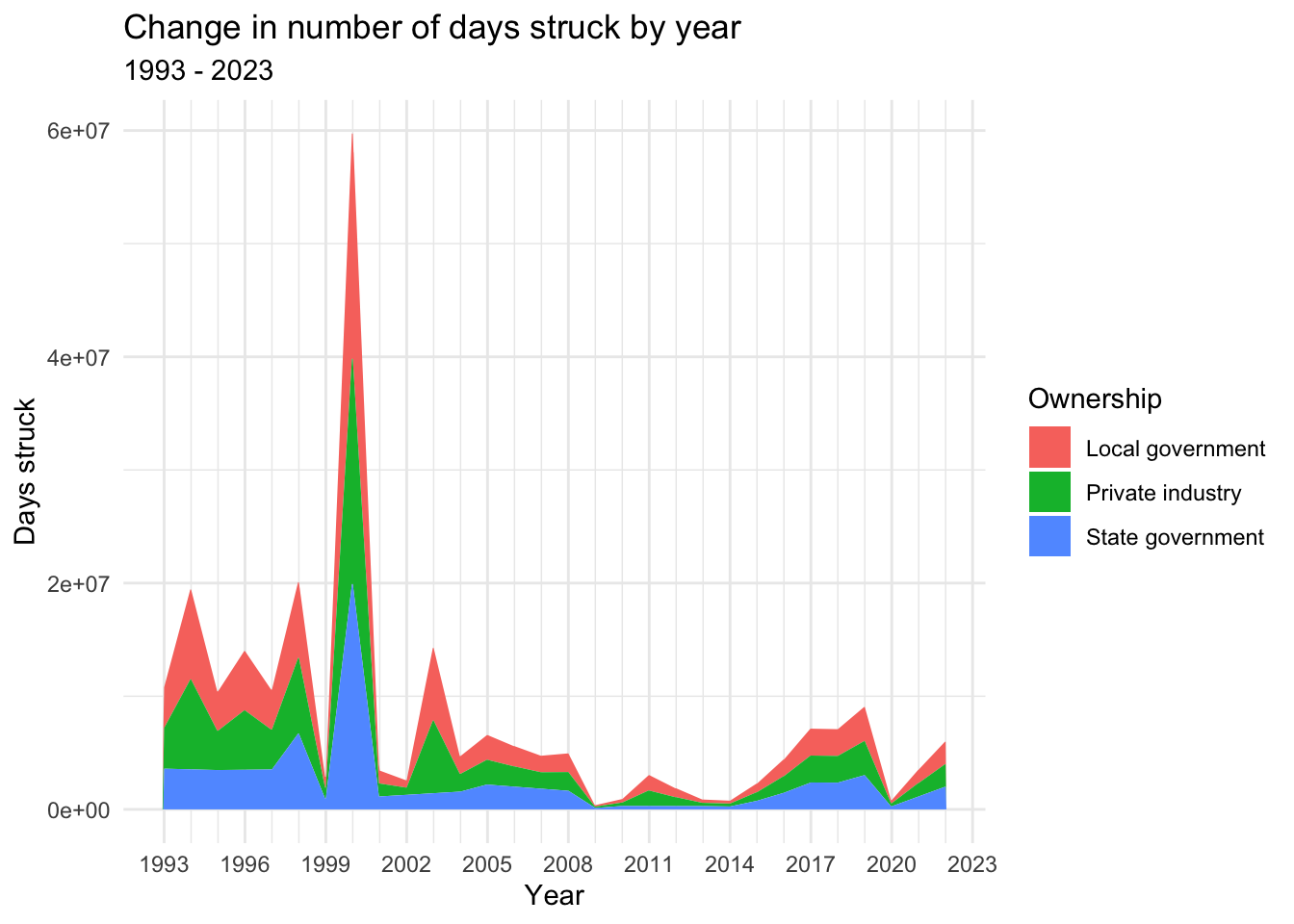

In all four graphs, we see relatively significant activity through the 1990s, until a sharp drop in 1999, followed by a large spike in 2000. Note that the 2000 spike is particularly massive in the Days struck visualizations, suggesting the presence of many very long strikes in that year.

After 2000, we see a period of decline with relatively little activity through the mid-2010s. Then, however, we find the largest spikes in the Workers graphs in 2018 and 2019, with large but not quite as significant spikes at that time in the Days struck graphs, suggesting the presence of very many relatively short strikes in these years. From there, we see a sharp drop in 2020—likely the result of the COVID-19 pandemic—followed by rises in the years after.

Highlight: 2000

To reiterate, 2000 features high in these views. Let’s go back to the un-condensed data and filter to strikes in 2000 with more than 5000 workers, sorted from most to least workers involved, to look at the most significant contributors.

Code

# create new data frame
strike00 <- strike

# change date to year
strike00$"Start date" <- as.numeric(format(strike00$"Start date", "%Y"))
strike00 <- strike00 %>%
  rename("Year" = "Start date") %>%
    
# filter to 2000, large strikes
  filter(Year==2000,Workers>5000) %>%
  select(Union,Employer,States,Areas,Workers,"Days struck")
strike00workers <- arrange(strike00, desc(Workers))

# view data
strike00workers

By far the largest strike in 2000, we see, was the commercial actors strike by the Screen Actors Guild (SAG) and the American Federation of Television and Radio Artists (AFTRA) against the American Association of Advertising Agencies, across most of the country.

The next largest strike in 2000 was by the Communication Workers of America (CWA) and the International Brotherhood of Electrical Workers (IBEW) against Verizon in the Northeast and Mid-Atlantic regions of the U.S.

Highlight: 2018 - 2019

Let’s do the same thing we did for 2000 with 2018 and 2019.

Code

# create new data frame
strike1819 <- strike

# change date to year
strike1819$"Start date" <- as.numeric(format(strike1819$"Start date", "%Y"))
strike1819 <- strike1819 %>%
  rename("Year" = "Start date") %>%
    
# filter to 2018, large strikes
  filter(Year==2018 | Year==2019,Workers>5000) %>%
  select(Union,Employer,States,Areas,Workers,"Days struck")
strike1819workers <- arrange(strike1819, desc(Workers))

# view data
strike1819workers

We see that many of the largest strikes in 2018 and 2019 were against state legislatures—particularly those of North Carolina, Arizona, Colorado, Oklahoma, West Virginia, Kentucky, Oregon, and South Carolina. These strikes, along with the strike against the Los Angeles Unified School District, made up the “#RedForEd” wave of teacher strikes in these years, named for the social media hashtag that accompanied it, referring to the red shirts striking teachers wore.

Changes in individual strike magnitude

Let’s look at the data in un-grouped form create a scatter lot of number of workers in strikes by start date.

Code

ggplot(strike, aes(x=as.Date(`Start date`))) +
  geom_point(aes(y=Workers),color="red",alpha=0.5) +
  scale_x_date(limits = as.Date(c("1993-01-01", "2023-01-01"))) +
  labs(title="Change in size of individual strikes by number of workers",subtitle="1993 - 2023",x="Year",y="# of workers striking")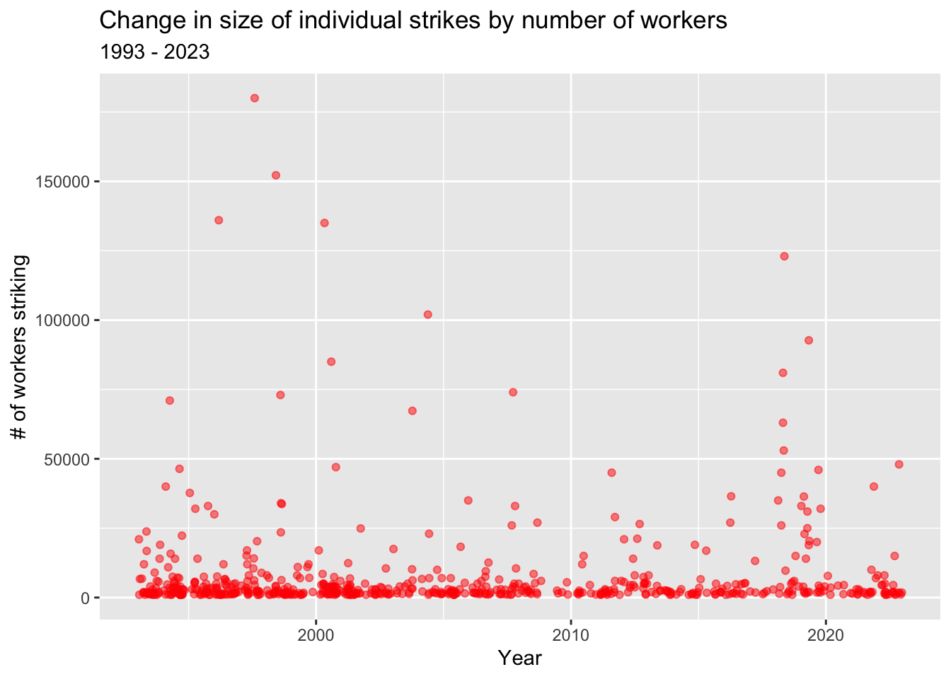

There is not much of a visible trend, though mid-size to large strikes do seem more concentrated before the early 2000s compared with after.

Private vs. public sector

How have strikes changed in size within the private sector and within the public sector (state government and local government), viewed separately? Let’s look at the same data as above but faceted by ownership type.

Code

ggplot(strike_own, aes(x=as.Date(`Start date`))) +
  geom_point(aes(y=Workers),color="red",alpha=0.5) +
  scale_x_date(limits = as.Date(c("1993-01-01", "2023-01-01"))) +
  facet_wrap(vars(Ownership)) +
  labs(title="Change in size of individual strikes by number of workers",subtitle="Separated by employer ownership type; 1993 - 2023",x="Year",y="# of workers striking")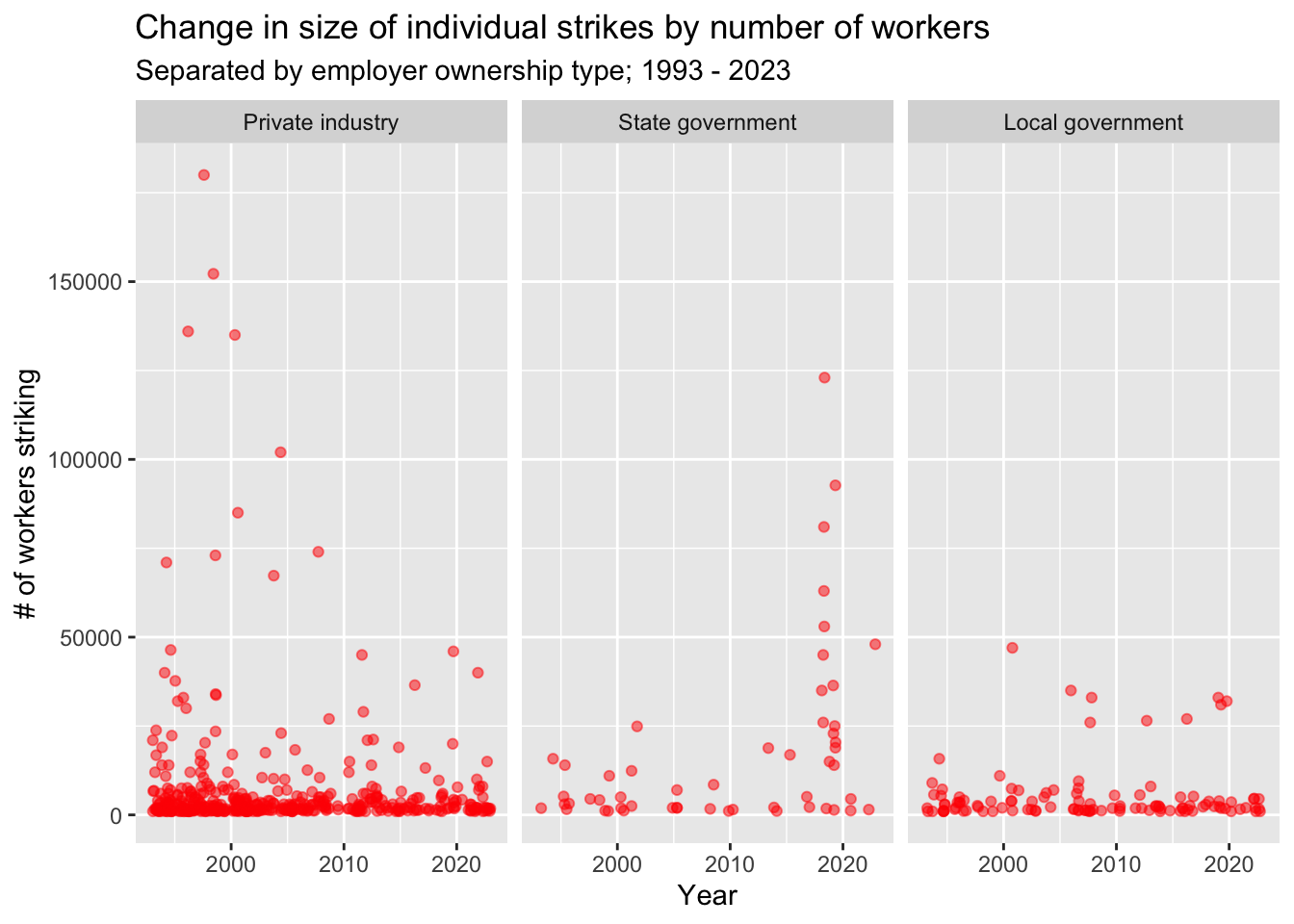

There appears to be a decrease in larger strikes in the private sector in the late 2000s, along with a sharp increase in larger strikes in state government in the late 2010s.

Conclusion

Though this project has provided valuable insights into the trends and characteristics of the labor movement in the United States over the past thirty years, there are still some questions it cannot answer. For instance, this analysis focuses primarily on quantitative aspects such as the number of workers involved and the duration of strikes, but it does not delve deeply into the underlying reasons and dynamics driving these strikes. Understanding the specific issues and demands of workers, as well as the responses of employers and the broader socio-political context, would require a more qualitative and comprehensive approach, such as conducting interviews or analyzing historical documents.

Through the process of putting together this project, I have discovered patterns and trends in strike activities over time, identified significant strikes in particular years, and examined differences between private and public sector strikes. It has become evident that strikes in the U.S. labor movement have experienced fluctuations in size and intensity, influenced by various factors such as economic conditions, union strength, and political climate. In particular, the 2000 and 2018/2019 strike waves stick out.

Exploring the qualitative aspects of strikes, such as the specific grievances and negotiation processes involved, would deepen our understanding of the labor movement’s dynamics. Additionally, analyzing the impact of strikes along with other types of labor action would contribute to a more comprehensive understanding of labor activism. By combining quantitative and qualitative approaches, future research can shed further light on the evolving nature of strikes and their role in shaping the labor landscape.

References

Bureau of Labor Statistics, U.S. Department of Labor. 2023a. “Union Members Summary - 2022 A01 Results.” January 19, 2023. https://www.bls.gov/news.release/union2.nr0.htm.

———. 2023b. “Work Stoppages, Detailed Monthly Listing, 2023.” https://www.bls.gov/wsp/publications/monthly-details/XLSX/work-stoppages-2023.xlsx.

Bureau of Labor Statistics, U.S. Department of Labor. n.d.a. “Work Stoppages, Detailed Monthly Listing, 2023.”

———. n.d.b. “Work Stoppages, Detailed Monthly Listing, 2023.”

R Core Team. 2023. R: A Language and Environment for Statistical Computing. Vienna, Austria: R Foundation for Statistical Computing. https://www.R-project.org/.

Wickham, Hadley, Mara Averick, Jennifer Bryan, Winston Chang, Lucy McGowan, Romain François, Garrett Grolemund, et al. 2019. “Welcome to the Tidyverse.” Journal of Open Source Software 4 (43): 1686. https://doi.org/10.21105/joss.01686.

Wickham, Hadley, and Jennifer Bryan. 2023. “Readxl: Read Excel Files.” https://readxl.tidyverse.org.

Wickham, Hadley, and Garrett Grolemund. 2017. R for Data Science. O’Reilly. https://r4ds.had.co.nz/index.html.

Introduction

Description of the data

Variables

Employer

States

Areas

Ownership

Union

Start date and End date

Workers

Days struck

How has labor militancy changed over the past 30 years?

Measures of central tendency

Changes in annual strike magnitude

Highlight: 2000

Highlight: 2018 - 2019

Changes in individual strike magnitude

Private vs. public sector

Conclusion

References

`Employer`

`States`

`Areas`

`Ownership`

`Union`

`Start date` and `End date`

`Workers`

`Days struck`